Rule build_renewable_profiles

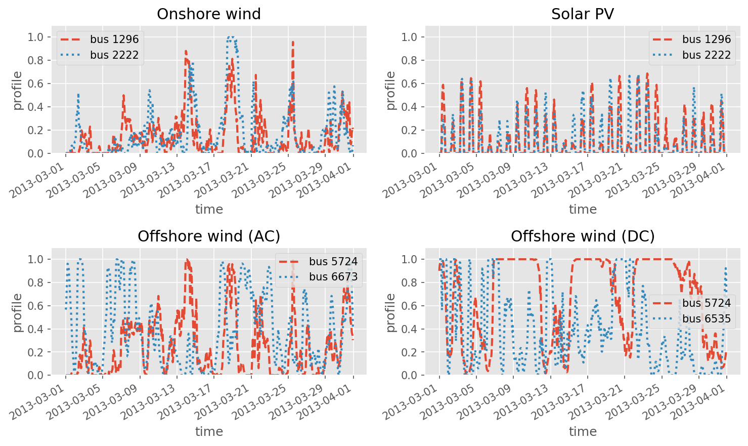
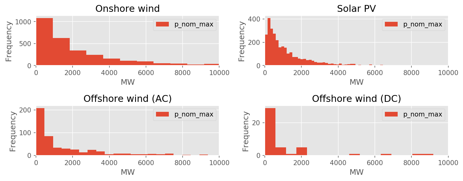
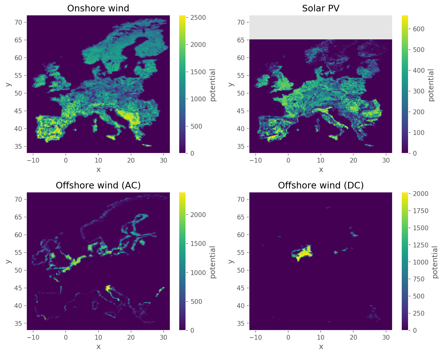
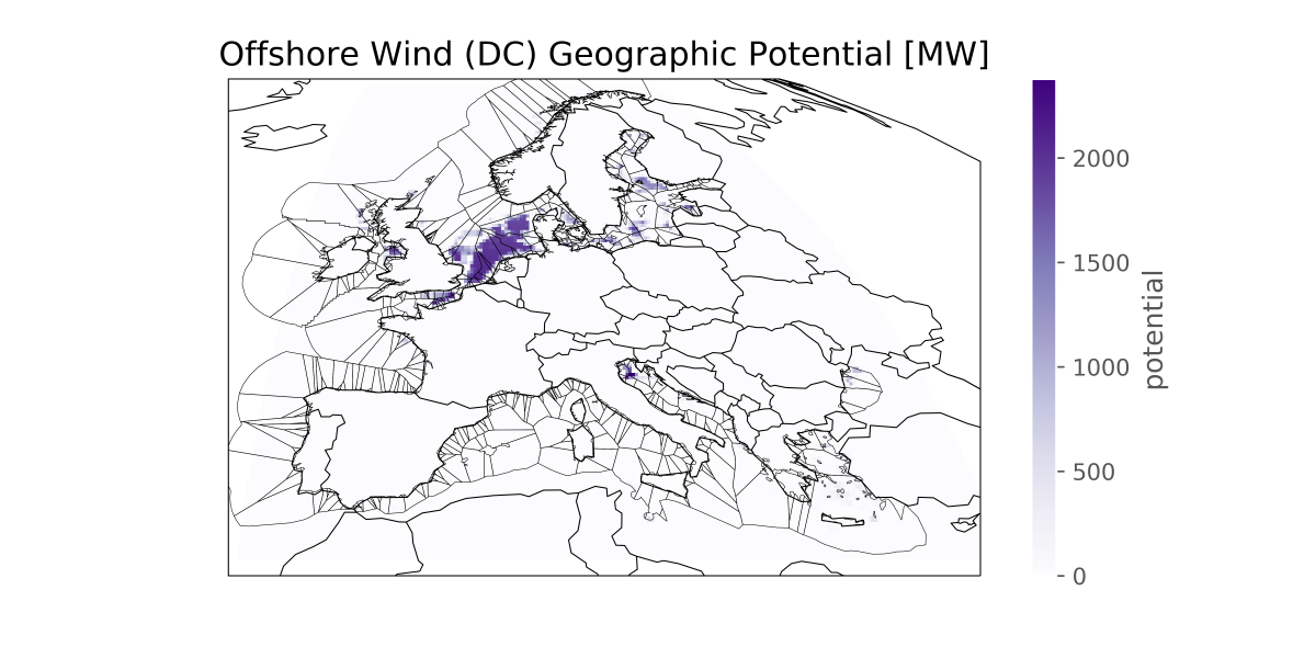
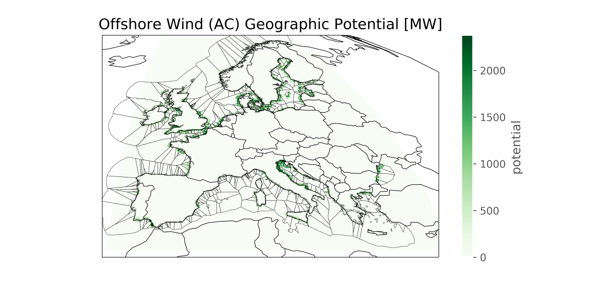
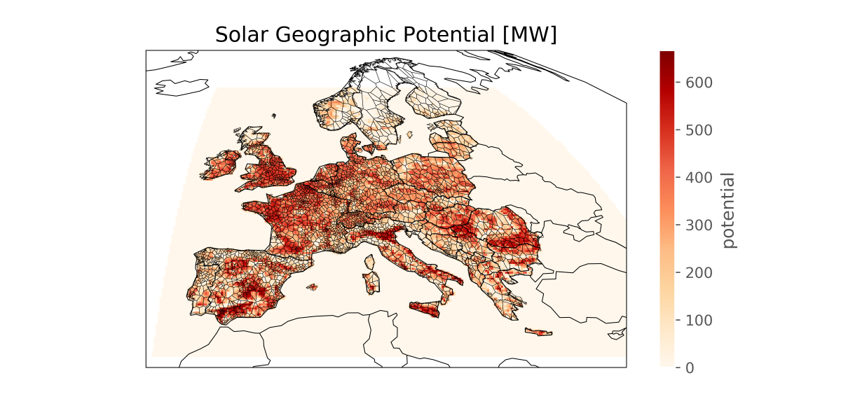
Calculates for each network node the (i) installable capacity (based on land- use), (ii) the available generation time series (based on weather data), and (iii) the average distance from the node for onshore wind, AC-connected offshore wind, DC-connected offshore wind and solar PV generators. For hydro generators, it calculates the expected inflows. In addition for offshore wind it calculates the fraction of the grid connection which is under water.

Relevant settings

snapshots:

atlite:
    nprocesses:

renewable:
    {technology}:
        cutout:
        copernicus:
            grid_codes:
            distance:
            distance_grid_codes:
        natura:
        max_depth:
        max_shore_distance:
        min_shore_distance:
        capacity_per_sqkm:
        correction_factor:
        potential:
        min_p_max_pu:
        clip_p_max_pu:
        resource:
        clip_min_inflow:

See also

Documentation of the configuration file config.yaml at snapshots, atlite, renewable

Inputs

• data/copernicus/PROBAV_LC100_global_v3.0.1_2019-nrt_Discrete-Classification-map_EPSG-4326.tif: Copernicus Land Service inventory on 23 land use classes (e.g. forests, arable land, industrial, urban areas) based on UN-FAO classification. See Table 4 in the PUM for a list of all classes.

  

• data/gebco/GEBCO_2021_TID.nc: A bathymetric data set with a global terrain model for ocean and land at 15 arc-second intervals by the General Bathymetric Chart of the Oceans (GEBCO).

  

  Source: GEBCO

• resources/natura.tiff: confer Rule build_natura_raster

• resources/offshore_shapes.geojson: confer Rule build_shapes

• resources/.geojson: (if not offshore wind), confer Rule build_bus_regions

• resources/regions_offshore.geojson: (if offshore wind), Rule build_bus_regions

• "cutouts/" + config["renewable"][{technology}]['cutout']: Rule build_cutout

• networks/base.nc: Rule base_network

Outputs

• resources/profile_{technology}.nc, except hydro technology, with the following structure

  Field	Dimensions	Description
  profile	bus, time	the per unit hourly availability factors for each node
  weight	bus	sum of the layout weighting for each node
  p_nom_max	bus	maximal installable capacity at the node (in MW)
  potential	y, x	layout of generator units at cutout grid cells inside the Voronoi cell (maximal installable capacity at each grid cell multiplied by capacity factor)
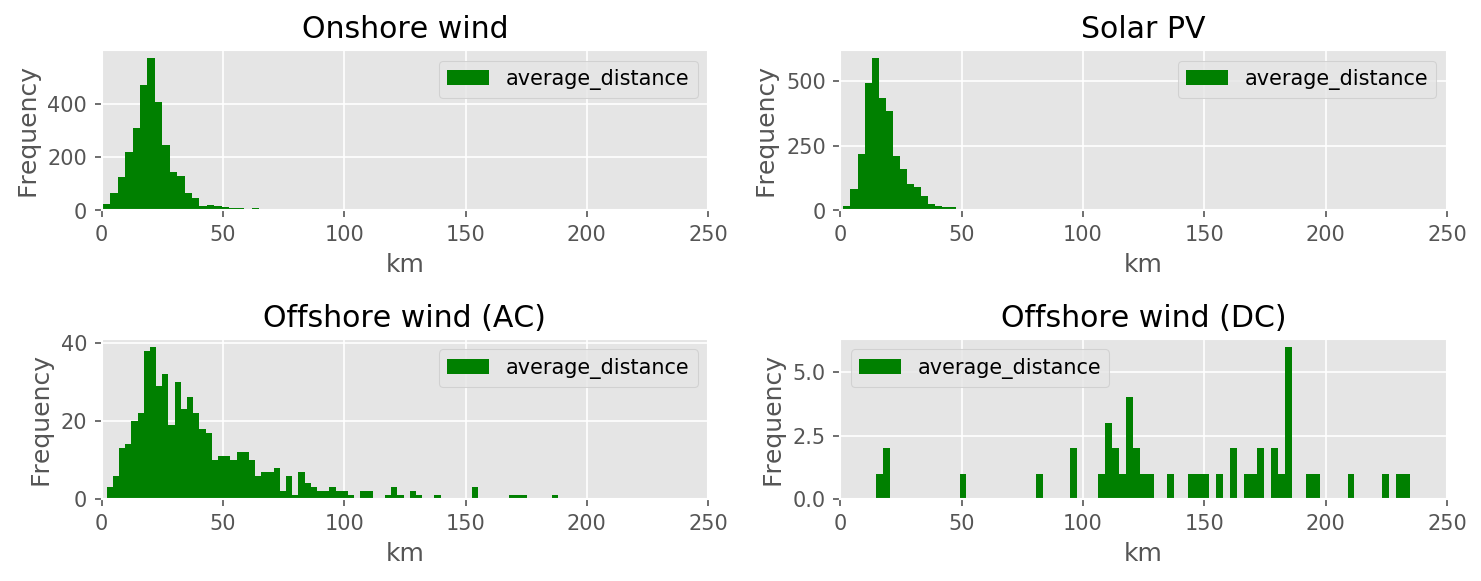
  average_distance	bus	average distance of units in the Voronoi cell to the grid node (in km)
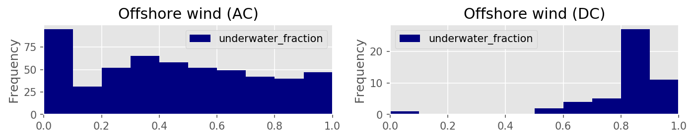
  underwater_fraction	bus	fraction of the average connection distance which is under water (only for offshore)

• resources/profile_hydro.nc for the hydro technology

  Field	Dimensions	Description
  inflow	plant, time	Inflow to the state of charge (in MW), e.g. due to river inflow in hydro reservoir.

  • profile

  

  • p_nom_max

  

  • potential

  

  • average_distance

  

  • underwater_fraction

  

Description

This script leverages on atlite function to derivate hourly time series for an entire year for solar, wind (onshore and offshore), and hydro data.

This script functions at two main spatial resolutions: the resolution of the network nodes and their Voronoi cells, and the resolution of the cutout grid cells for the weather data. Typically the weather data grid is finer than the network nodes, so we have to work out the distribution of generators across the grid cells within each Voronoi cell. This is done by taking account of a combination of the available land at each grid cell and the capacity factor there.

This uses the Copernicus land use data, Natura2000 nature reserves and GEBCO bathymetry data.

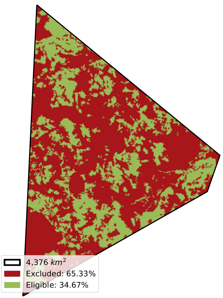
To compute the layout of generators in each node’s Voronoi cell, the installable potential in each grid cell is multiplied with the capacity factor at each grid cell. This is done since we assume more generators are installed at cells with a higher capacity factor.

This layout is then used to compute the generation availability time series from the weather data cutout from atlite.

Two methods are available to compute the maximal installable potential for the node (p_nom_max): simple and conservative:

• simple adds up the installable potentials of the individual grid cells. If the model comes close to this limit, then the time series may slightly overestimate production since it is assumed the geographical distribution is proportional to capacity factor.

• conservative ascertains the nodal limit by increasing capacities proportional to the layout until the limit of an individual grid cell is reached.