API Reference (automated)#
_helpers#
- _helpers.configure_logging(snakemake, skip_handlers=False)#
Configure the basic behaviour for the logging module.
Note: Must only be called once from the __main__ section of a script.
The setup includes printing log messages to STDERR and to a log file defined by either (in priority order): snakemake.log.python, snakemake.log[0] or “logs/{rulename}.log”. Additional keywords from logging.basicConfig are accepted via the snakemake configuration file under snakemake.config.logging.
- Parameters:
snakemake (snakemake object) – Your snakemake object containing a snakemake.config and snakemake.log.
skip_handlers (True | False (default)) – Do (not) skip the default handlers created for redirecting output to STDERR and file.
- _helpers.country_name_2_two_digits(country_name)#
Convert full country name to 2-digit country code.
- _helpers.create_country_list(input, iso_coding=True)#
Create a country list for defined regions..
- Parameters:
input (str) – Any two-letter country name, regional name, or continent given in the regions config file. Country name duplications won’t distort the result. Examples are: [“NG”,”ZA”], downloading osm data for Nigeria and South Africa [“africa”], downloading data for Africa [“NAR”], downloading data for the North African Power Pool [“TEST”], downloading data for a customized test set. [“NG”,”ZA”,”NG”], won’t distort result.
- Returns:
full_codes_list – Example [“NG”,”ZA”]
- Return type:
- _helpers.create_logger(logger_name, level=20)#
Create a logger for a module and adds a handler needed to capture in logs traceback from exceptions emerging during the workflow.
- _helpers.get_aggregation_strategies(aggregation_strategies)#
Default aggregation strategies that cannot be defined in .yaml format must be specified within the function, otherwise (when defaults are passed in the function’s definition) they get lost when custom values are specified in the config.
- _helpers.get_last_commit_message(path)#
Function to get the last PyPSA-Earth Git commit message.
- Returns:
result
- Return type:
string
- _helpers.handle_exception(exc_type, exc_value, exc_traceback)#
Customise errors traceback.
- _helpers.load_network(import_name=None, custom_components=None)#
Helper for importing a pypsa.Network with additional custom components.
- Parameters:
import_name (str) – As in pypsa.Network(import_name)
custom_components (dict) –
Dictionary listing custom components. For using
snakemake.params.override_components"]inconfig.yamldefine:override_components: ShadowPrice: component: ["shadow_prices","Shadow price for a global constraint.",np.nan] attributes: name: ["string","n/a","n/a","Unique name","Input (required)"] value: ["float","n/a",0.,"shadow value","Output"]
- Return type:
pypsa.Network
- _helpers.mock_snakemake(rulename, **wildcards)#
This function is expected to be executed from the “scripts”-directory of ” the snakemake project. It returns a snakemake.script.Snakemake object, based on the Snakefile.
If a rule has wildcards, you have to specify them in wildcards.
- Parameters:
rulename (str) – name of the rule for which the snakemake object should be generated
wildcards – keyword arguments fixing the wildcards. Only necessary if wildcards are needed.
- _helpers.progress_retrieve(url, file, data=None, headers=None, disable_progress=False, roundto=1.0)#
Function to download data from a url with a progress bar progress in retrieving data.
- Parameters:
url (str) – Url to download data from
file (str) – File where to save the output
data (dict) – Data for the request (default None), when not none Post method is used
disable_progress (bool) – When true, no progress bar is shown
roundto (float) – (default 0) Precision used to report the progress e.g. 0.1 stands for 88.1, 10 stands for 90, 80
- _helpers.read_csv_nafix(file, **kwargs)#
Function to open a csv as pandas file and standardize the na value
- _helpers.read_geojson(fn, cols=[], dtype=None, crs='EPSG:4326')#
Function to read a geojson file fn. When the file is empty, then an empty GeoDataFrame is returned having columns cols, the specified crs and the columns specified by the dtype dictionary it not none.
Parameters:#
- fnstr
Path to the file to read
- colslist
List of columns of the GeoDataFrame
- dtypedict
Dictionary of the type of the object by column
- crsstr
CRS of the GeoDataFrame
- _helpers.read_osm_config(*args)#
Read values from the regions config file based on provided key arguments.
- Parameters:
*args (str) – One or more key arguments corresponding to the values to retrieve from the config file. Typical arguments include “world_iso”, “continent_regions”, “iso_to_geofk_dict”, and “osm_clean_columns”.
- Returns:
If a single key is provided, returns the corresponding value from the regions config file. If multiple keys are provided, returns a tuple containing values corresponding to the provided keys.
- Return type:
Examples
>>> values = read_osm_config("key1", "key2")
>>> print(values)
('value1', 'value2')
>>> world_iso = read_osm_config("world_iso")
>>> print(world_iso)
{"Africa": {"DZ": "algeria", ...}, ...}
- _helpers.sets_path_to_root(root_directory_name)#
Search and sets path to the given root directory (root/path/file).
- _helpers.three_2_two_digits_country(three_code_country)#
Convert 3-digit to 2-digit country code:
- _helpers.two_2_three_digits_country(two_code_country)#
Convert 2-digit to 3-digit country code:
- _helpers.two_digits_2_name_country(two_code_country, nocomma=False, remove_start_words=[])#
Convert 2-digit country code to full name country:
- Parameters:
two_code_country (str) – 2-digit country name
nocomma (bool (optional, default False)) – When true, country names with comma are extended to remove the comma. Example CD -> Congo, The Democratic Republic of -> The Democratic Republic of Congo
remove_start_words (list (optional, default empty)) – When a sentence starts with any of the provided words, the beginning is removed. e.g. The Democratic Republic of Congo -> Democratic Republic of Congo (remove_start_words=[“The”])
- Returns:
full_name – full country name
- Return type:
add_electricity#
Adds electrical generators, load and existing hydro storage units to a base network.
Relevant Settings#
costs:
    year:
    version:
    rooftop_share:
    USD2013_to_EUR2013:
    dicountrate:
    emission_prices:

electricity:
    max_hours:
    marginal_cost:
    capital_cost:
    conventional_carriers:
    co2limit:
    extendable_carriers:
    include_renewable_capacities_from_OPSD:
    estimate_renewable_capacities_from_capacity_stats:

renewable:
    hydro:
        carriers:
        hydro_max_hours:
        hydro_max_hours_default:
        hydro_capital_cost:

lines:
    length_factor:
See also
Documentation of the configuration file config.yaml at costs,
electricity, load_options, renewable, lines
Inputs#
resources/costs.csv: The database of cost assumptions for all included technologies for specific years from various sources; e.g. discount rate, lifetime, investment (CAPEX), fixed operation and maintenance (FOM), variable operation and maintenance (VOM), fuel costs, efficiency, carbon-dioxide intensity.data/bundle/hydro_capacities.csv: Hydropower plant store/discharge power capacities, energy storage capacity, and average hourly inflow by country. Not currently used!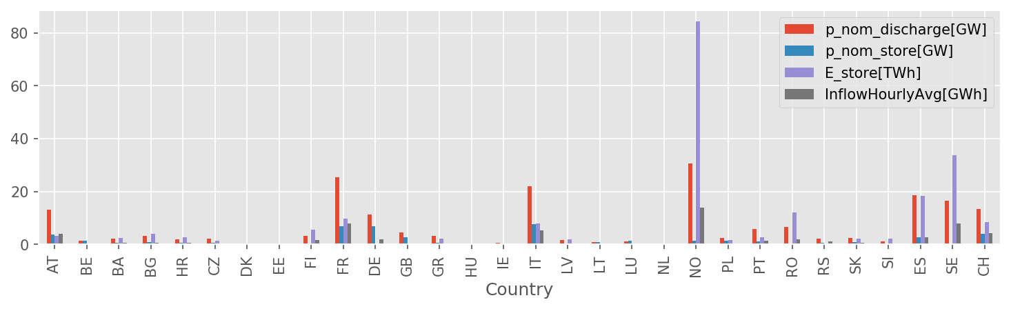
data/geth2015_hydro_capacities.csv: alternative to capacities above; not currently used!resources/demand_profiles.csv: a csv file containing the demand profile associated with busesresources/shapes/gadm_shapes.geojson: confer Rule build_shapesresources/powerplants.csv: confer Rule build_powerplantsresources/profile_{}.nc: all technologies inconfig["renewables"].keys(), confer Rule build_renewable_profilesnetworks/base.nc: confer Rule base_network
Outputs#
networks/elec.nc: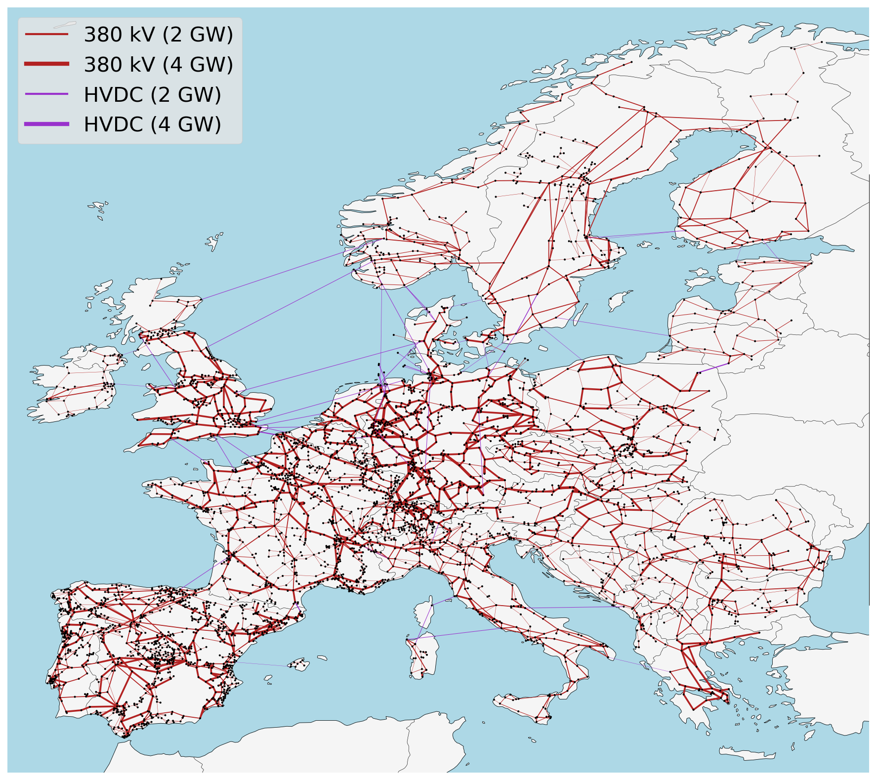
Description#
The rule add_electricity ties all the different data inputs from the preceding rules together into a detailed PyPSA network that is stored in networks/elec.nc. It includes:
today’s transmission topology and transfer capacities (in future, optionally including lines which are under construction according to the config settings
lines: under_constructionandlinks: under_construction),today’s thermal and hydro power generation capacities (for the technologies listed in the config setting
electricity: conventional_carriers), andtoday’s load time-series (upsampled in a top-down approach according to population and gross domestic product)
It further adds extendable generators with zero capacity for
photovoltaic, onshore and AC- as well as DC-connected offshore wind installations with today’s locational, hourly wind and solar capacity factors (but no current capacities),
additional open- and combined-cycle gas turbines (if
OCGTand/orCCGTis listed in the config settingelectricity: extendable_carriers)
- add_electricity.attach_load(n, demand_profiles)#
Add load profiles to network buses.
- Parameters:
n (pypsa network)
demand_profiles (str) – Path to csv file of elecric demand time series, e.g. “resources/demand_profiles.csv” Demand profile has snapshots as rows and bus names as columns.
- Returns:
n – Now attached with load time series
- Return type:
pypsa network
- add_electricity.calculate_annuity(n, r)#
Calculate the annuity factor for an asset with lifetime n years and discount rate of r, e.g. annuity(20, 0.05) * 20 = 1.6.
- add_electricity.load_costs(tech_costs, config, elec_config, Nyears=1)#
Set all asset costs and other parameters.
base_network#
Creates the network topology from a OpenStreetMap.
Relevant Settings#
snapshots:

countries:

electricity:
    voltages:

lines:
    types:
    s_max_pu:
    under_construction:

links:
    p_max_pu:
    p_nom_max:
    under_construction:

transformers:
    x:
    s_nom:
    type:
See also
Documentation of the configuration file config.yaml at
snapshots, Top-level configuration, electricity, load_options,
lines, links, transformers
Inputs#
Outputs#
networks/base.nc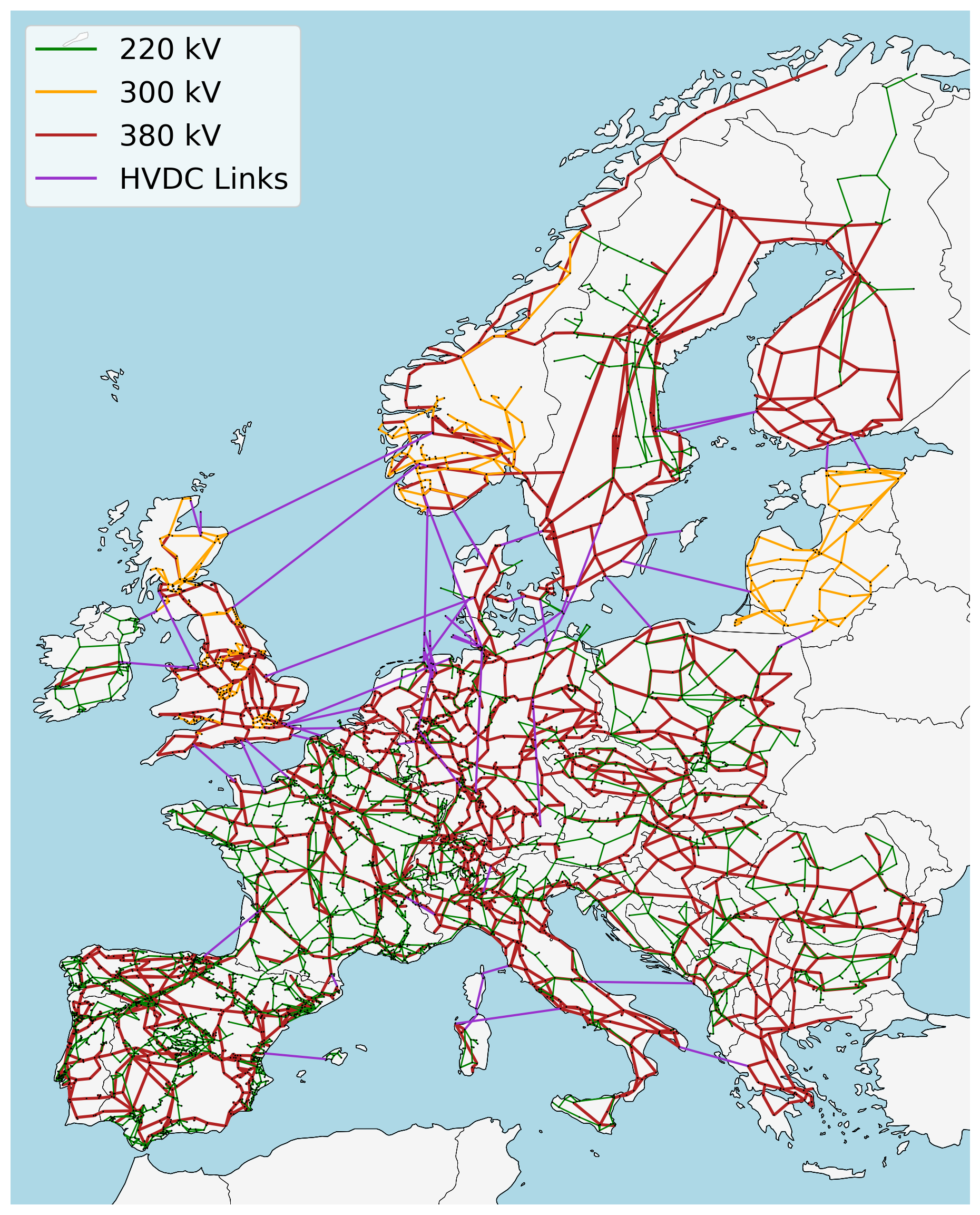
Description#
build_bus_regions#
Creates Voronoi shapes for each bus representing both onshore and offshore regions.
Relevant Settings#
countries:
See also
Documentation of the configuration file config.yaml at
Top-level configuration
Inputs#
resources/country_shapes.geojson: confer Rule build_shapesresources/offshore_shapes.geojson: confer Rule build_shapesnetworks/base.nc: confer Rule base_network
Outputs#
resources/regions_onshore.geojson: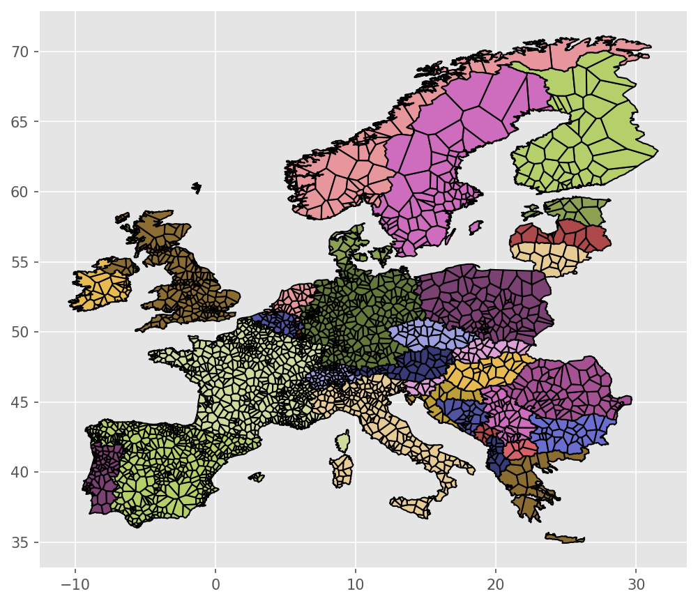
resources/regions_offshore.geojson: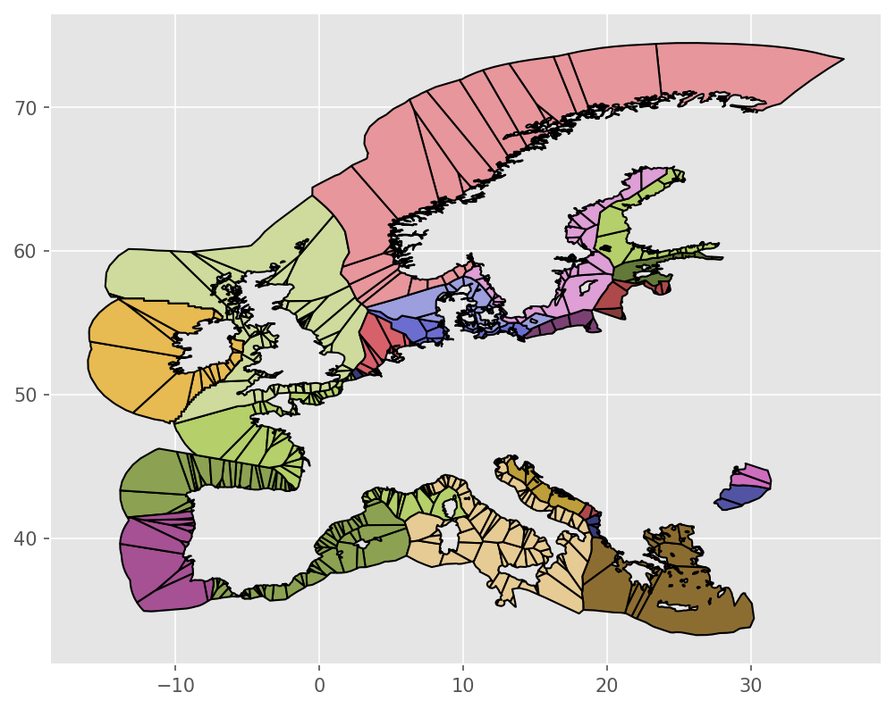
Description#
- build_bus_regions.custom_voronoi_partition_pts(points, outline, add_bounds_shape=True, multiplier=5)#
Compute the polygons of a voronoi partition of points within the polygon outline
- build_bus_regions.points#
- Type:
Nx2 - ndarray[dtype=float]
- build_bus_regions.outline#
- Type:
Polygon
- Returns:
polygons
- Return type:
N - ndarray[dtype=Polygon|MultiPolygon]
build_cutout#
Create cutouts with atlite.
For this rule to work you must have
installed the Copernicus Climate Data Store
cdsapipackage (install with `pip`) andregistered and setup your CDS API key as described on their website. The CDS API allows an automatic filedownload by executing this script
See also
For details on the weather data read the atlite documentation. If you need help specifically for creating cutouts the corresponding section in the atlite documentation should be helpful.
Relevant Settings#
atlite:
    nprocesses:
    cutouts:
        {cutout}:
See also
Documentation of the configuration file config.yaml at
atlite
Inputs#
None
Outputs#
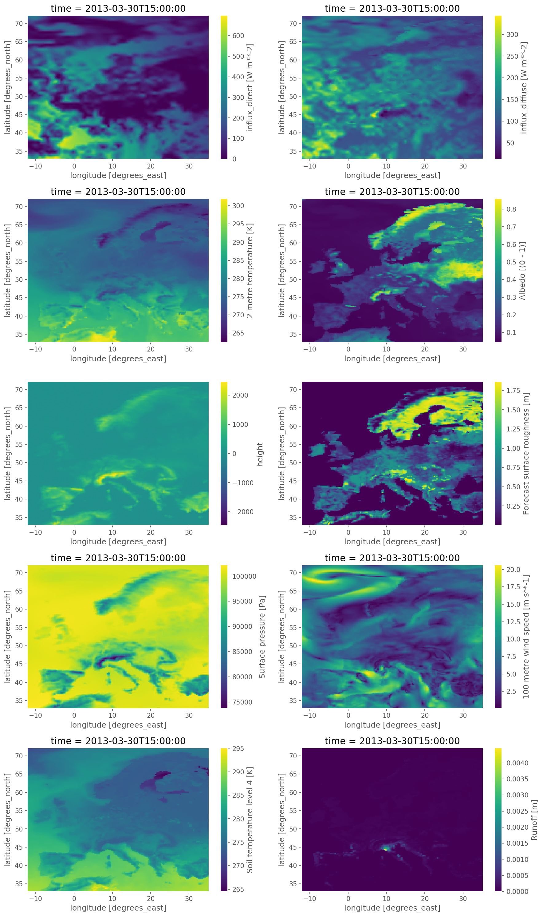
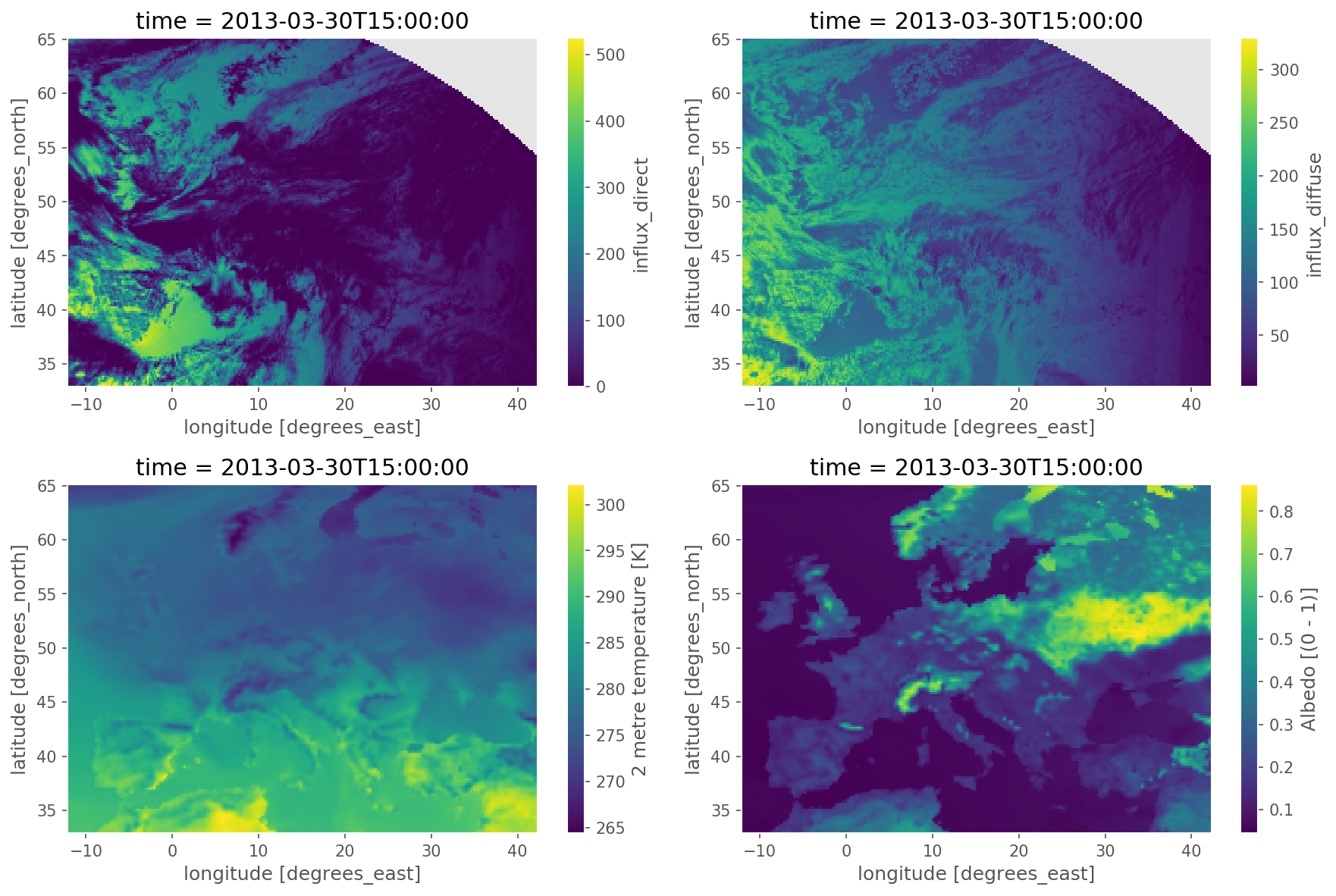
cutouts/{cutout}: weather data from either the ERA5 reanalysis weather dataset or SARAH-2 satellite-based historic weather data with the following structure:
ERA5 cutout:
Field
Dimensions
Unit
Description
pressure
time, y, x
Pa
Surface pressure
temperature
time, y, x
K
Air temperature 2 meters above the surface.
soil temperature
time, y, x
K
Soil temperature between 1 meters and 3 meters depth (layer 4).
influx_toa
time, y, x
Wm**-2
Top of Earth’s atmosphere TOA incident solar radiation
influx_direct
time, y, x
Wm**-2
Total sky direct solar radiation at surface
runoff
time, y, x
m
Runoff (volume per area)
roughness
y, x
m
Forecast surface roughness (roughness length)
height
y, x
m
Surface elevation above sea level
albedo
time, y, x
–
Albedo measure of diffuse reflection of solar radiation. Calculated from relation between surface solar radiation downwards (Jm**-2) and surface net solar radiation (Jm**-2). Takes values between 0 and 1.
influx_diffuse
time, y, x
Wm**-2
Diffuse solar radiation at surface. Surface solar radiation downwards minus direct solar radiation.
wnd100m
time, y, x
ms**-1
Wind speeds at 100 meters (regardless of direction)
A SARAH-2 cutout can be used to amend the fields temperature, influx_toa, influx_direct, albedo,
influx_diffuse of ERA5 using satellite-based radiation observations.
Description#
build_demand_profiles#
Creates electric demand profile csv.
Relevant Settings#
load:
    scale:
    ssp:
    weather_year:
    prediction_year:
    region_load:
Inputs#
networks/base.nc: confer Rule base_network, a base PyPSA Networkresources/bus_regions/regions_onshore.geojson: conferbuild_bus_regionsload_data_paths: paths to load profiles, e.g. hourly country load profiles produced by GEGISresources/shapes/gadm_shapes.geojson: confer Rule build_shapes, file containing the gadm shapes
Outputs#
resources/demand_profiles.csv: the content of the file is the electric demand profile associated to each bus. The file has the snapshots as rows and the buses of the network as columns.
Description#
The rule build_demand creates load demand profiles in correspondence of the buses of the network.
It creates the load paths for GEGIS outputs by combining the input parameters of the countries, weather year, prediction year, and SSP scenario.
Then with a function that takes in the PyPSA network “base.nc”, region and gadm shape data, the countries of interest, a scale factor, and the snapshots,
it returns a csv file called “demand_profiles.csv”, that allocates the load to the buses of the network according to GDP and population.
- build_demand_profiles.build_demand_profiles(n, load_paths, regions, admin_shapes, countries, scale, start_date, end_date, out_path)#
Create csv file of electric demand time series.
- Parameters:
n (pypsa network)
load_paths (paths of the load files)
regions (.geojson) – Contains bus_id of low voltage substations and bus region shapes (voronoi cells)
admin_shapes (.geojson) – contains subregional gdp, population and shape data
countries (list) – List of countries that is config input
scale (float) – The scale factor is multiplied with the load (1.3 = 30% more load)
start_date (parameter) – The start_date is the first hour of the first day of the snapshots
end_date (parameter) – The end_date is the last hour of the last day of the snapshots
- Returns:
demand_profiles.csv
- Return type:
csv file containing the electric demand time series
- build_demand_profiles.get_gegis_regions(countries)#
Get the GEGIS region from the config file.
- build_demand_profiles.get_load_paths_gegis(ssp_parentfolder, config)#
Create load paths for GEGIS outputs.
The paths are created automatically according to included country, weather year, prediction year and ssp scenario
Example
[“/data/ssp2-2.6/2030/era5_2013/Africa.nc”, “/data/ssp2-2.6/2030/era5_2013/Africa.nc”]
- build_demand_profiles.shapes_to_shapes(orig, dest)#
Adopted from vresutils.transfer.Shapes2Shapes()
build_natura_raster#
Converts vectordata or known as shapefiles (i.e. used for geopandas/shapely) to our cutout rasters. The Protected Planet Data on protected areas is aggregated to all cutout regions.
Relevant Settings#
renewable:
    {technology}:
        cutout:
See also
Documentation of the configuration file config.yaml at
renewable
Inputs#
data/landcover/world_protected_areas/*.shp: shapefiles representing the world protected areas, such as the World Database of Protected Areas (WDPA).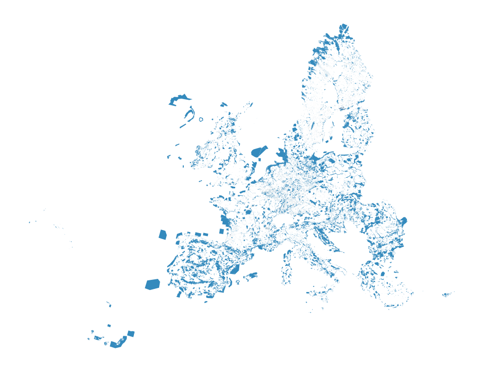
Outputs#
resources/natura/natura.tiff: Rasterized version of the world protected areas, such as WDPA natural protection areas to reduce computation times.
Description#
To operate the script you need all input files.
This script collects all shapefiles available in the folder data/landcover/* describing regions of protected areas, merges them to one shapefile, and create a rasterized version of the region, that covers the region described by the cutout. The output is a raster file with the name natura.tiff in the folder resources/natura/.
- build_natura_raster.get_fileshapes(list_paths, accepted_formats=('.shp',))#
Function to parse the list of paths to include shapes included in folders, if any
- build_natura_raster.unify_protected_shape_areas(inputs, natura_crs, out_logging)#
Iterates through all snakemake rule inputs and unifies shapefiles (.shp) only.
The input is given in the Snakefile and shapefiles are given by .shp
- Returns:
unified_shape
- Return type:
GeoDataFrame with a unified “multishape”
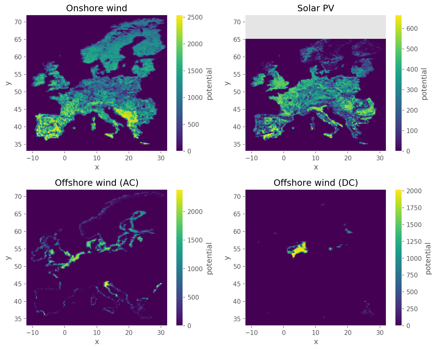
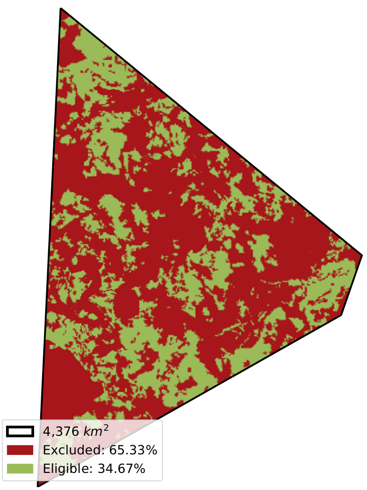
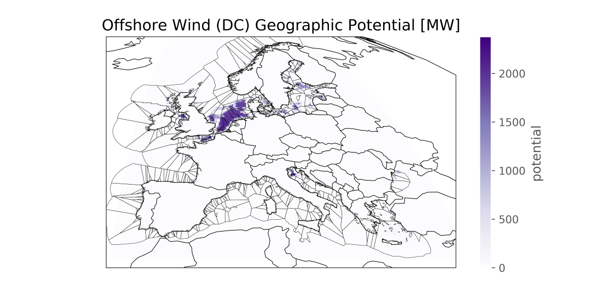
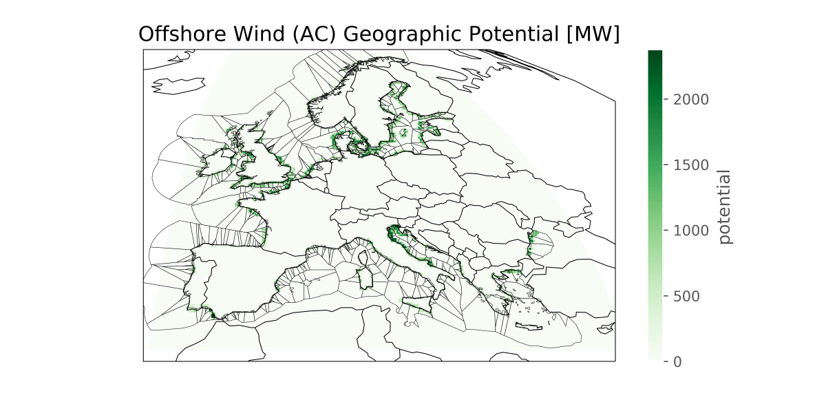
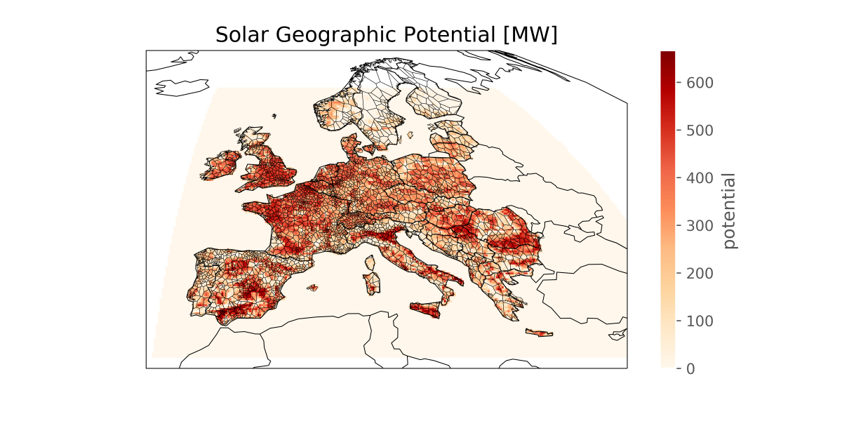
build_renewable_profiles#
Calculates for each network node the (i) installable capacity (based on land- use), (ii) the available generation time series (based on weather data), and (iii) the average distance from the node for onshore wind, AC-connected offshore wind, DC-connected offshore wind and solar PV generators. For hydro generators, it calculates the expected inflows. In addition for offshore wind it calculates the fraction of the grid connection which is under water.
Relevant settings#
snapshots:

atlite:
    nprocesses:

renewable:
    {technology}:
        cutout:
        copernicus:
            grid_codes:
            distance:
            distance_grid_codes:
        natura:
        max_depth:
        max_shore_distance:
        min_shore_distance:
        capacity_per_sqkm:
        correction_factor:
        potential:
        min_p_max_pu:
        clip_p_max_pu:
        resource:
        clip_min_inflow:
Inputs#
data/copernicus/PROBAV_LC100_global_v3.0.1_2019-nrt_Discrete-Classification-map_EPSG-4326.tif: Copernicus Land Service inventory on 23 land use classes (e.g. forests, arable land, industrial, urban areas) based on UN-FAO classification. See Table 4 in the PUM for a list of all classes.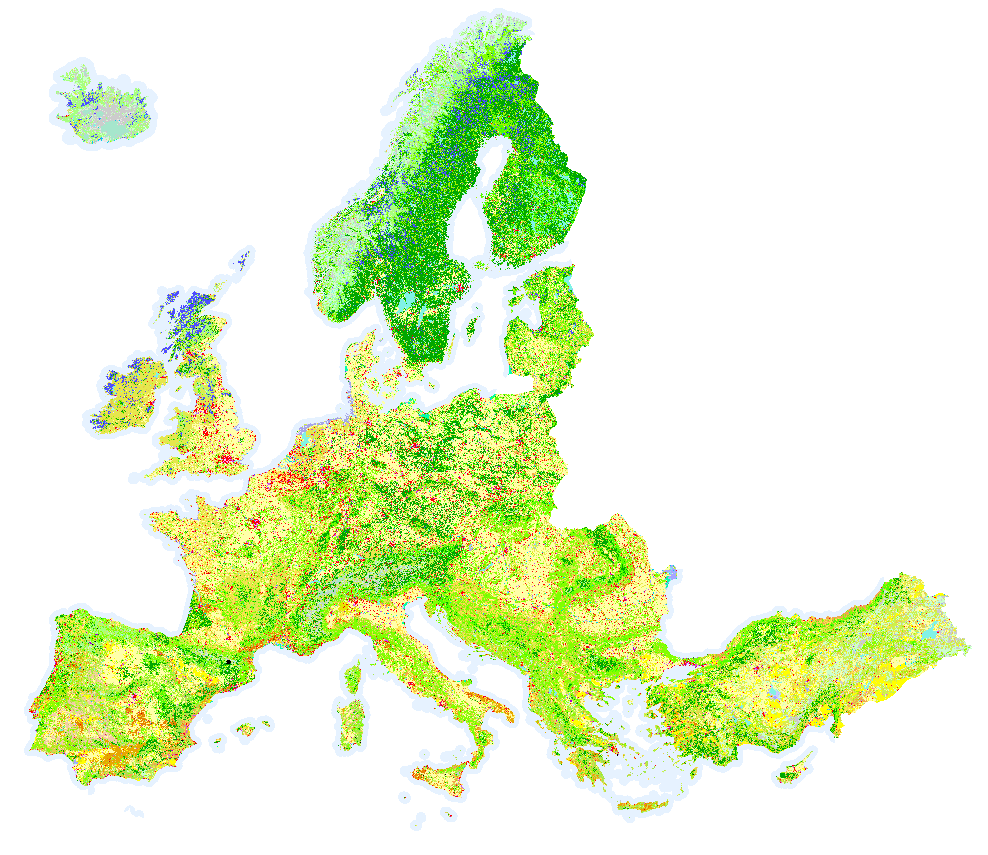
data/gebco/GEBCO_2021_TID.nc: A bathymetric data set with a global terrain model for ocean and land at 15 arc-second intervals by the General Bathymetric Chart of the Oceans (GEBCO).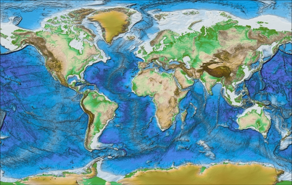
Source: GEBCO
resources/natura.tiff: confer Rule build_natura_rasterresources/offshore_shapes.geojson: confer Rule build_shapesresources/.geojson: (if not offshore wind), confer Rule build_bus_regionsresources/regions_offshore.geojson: (if offshore wind), Rule build_bus_regions"cutouts/" + config["renewable"][{technology}]['cutout']: Rule build_cutoutnetworks/base.nc: Rule base_network
Outputs#
resources/profile_{technology}.nc, except hydro technology, with the following structureField
Dimensions
Description
profile
bus, time
the per unit hourly availability factors for each node
weight
bus
sum of the layout weighting for each node
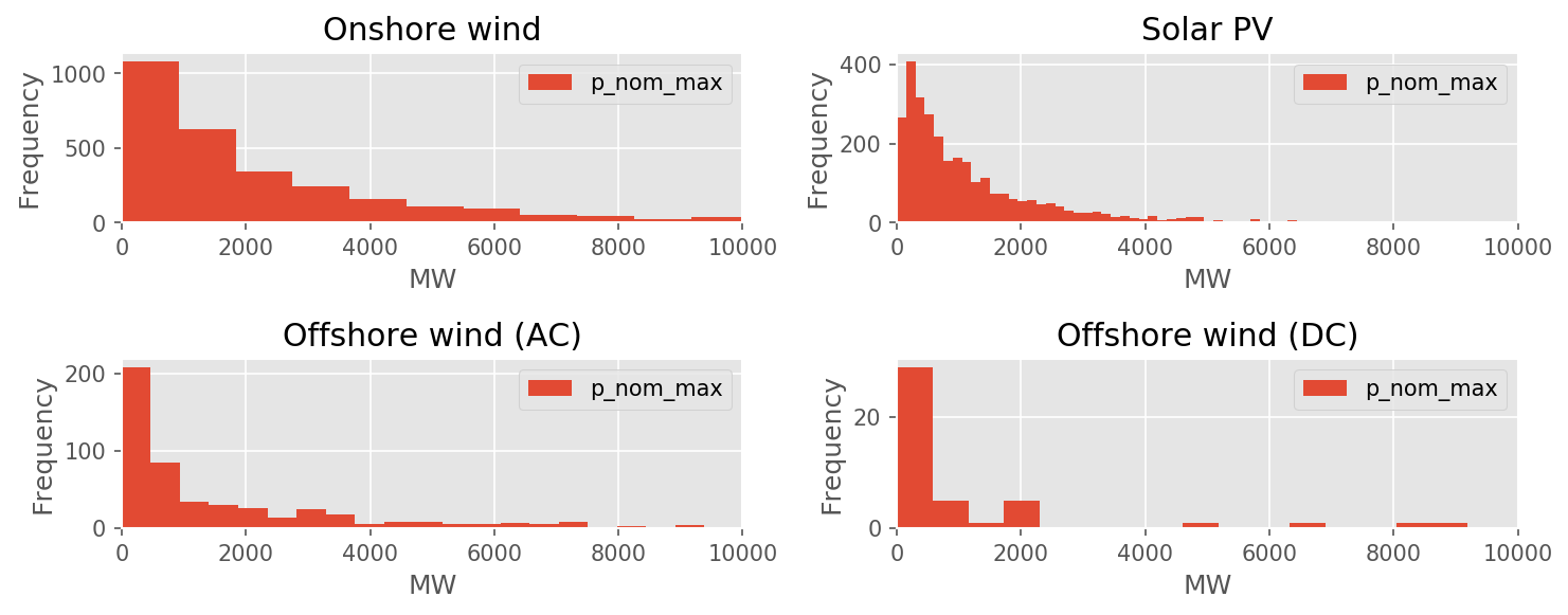
p_nom_max
bus
maximal installable capacity at the node (in MW)
potential
y, x
layout of generator units at cutout grid cells inside the Voronoi cell (maximal installable capacity at each grid cell multiplied by capacity factor)
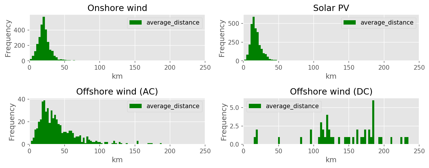
average_distance
bus
average distance of units in the Voronoi cell to the grid node (in km)
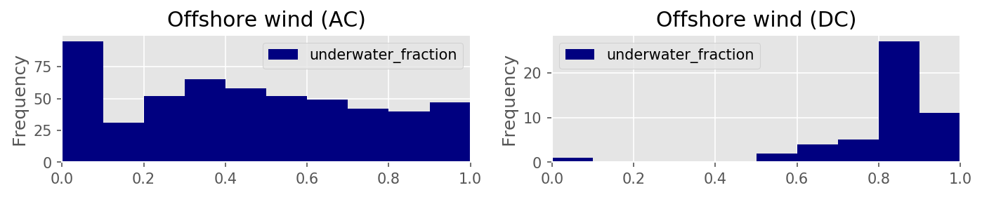
underwater_fraction
bus
fraction of the average connection distance which is under water (only for offshore)
resources/profile_hydro.ncfor the hydro technologyField
Dimensions
Description
inflow
plant, time
Inflow to the state of charge (in MW), e.g. due to river inflow in hydro reservoir.
profile
p_nom_max
potential
average_distance
underwater_fraction
Description#
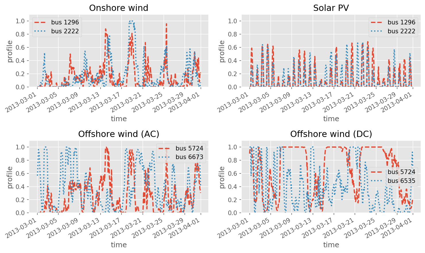
This script leverages on atlite function to derivate hourly time series for an entire year for solar, wind (onshore and offshore), and hydro data.
This script functions at two main spatial resolutions: the resolution of the network nodes and their Voronoi cells, and the resolution of the cutout grid cells for the weather data. Typically the weather data grid is finer than the network nodes, so we have to work out the distribution of generators across the grid cells within each Voronoi cell. This is done by taking account of a combination of the available land at each grid cell and the capacity factor there.
This uses the Copernicus land use data, Natura2000 nature reserves and GEBCO bathymetry data.
To compute the layout of generators in each node’s Voronoi cell, the installable potential in each grid cell is multiplied with the capacity factor at each grid cell. This is done since we assume more generators are installed at cells with a higher capacity factor.

This layout is then used to compute the generation availability time series
from the weather data cutout from atlite.
Two methods are available to compute the maximal installable potential for the
node (p_nom_max): simple and conservative:
simpleadds up the installable potentials of the individual grid cells. If the model comes close to this limit, then the time series may slightly overestimate production since it is assumed the geographical distribution is proportional to capacity factor.conservativeascertains the nodal limit by increasing capacities proportional to the layout until the limit of an individual grid cell is reached.
- build_renewable_profiles.check_cutout_completness(cf)#
Check if a cutout contains missed values.
That may be the case due to some issues with accessibility of ERA5 data See for details https://confluence.ecmwf.int/display/CUSF/Missing+data+in+ERA5T Returns share of cutout cells with missed data
- build_renewable_profiles.estimate_bus_loss(data_column, tech)#
Calculated share of buses with data loss due to flaws in the cutout data.
Returns share of the buses with missed data
- build_renewable_profiles.filter_cutout_region(cutout, regions)#
Filter the cutout to focus on the region of interest.
- build_renewable_profiles.rescale_hydro(plants, runoff, normalize_using_yearly, normalization_year)#
Function used to rescale the inflows of the hydro capacities to match country statistics.
- Parameters:
plants (DataFrame) – Run-of-river plants orf dams with lon, lat, countries, installed_hydro columns. Countries and installed_hydro column are only used with normalize_using_yearly installed_hydro column shall be a boolean vector specifying whether that plant is currently installed and used to normalize the inflows
runoff (xarray object) – Runoff at each bus
normalize_using_yearly (DataFrame) – Dataframe that specifies for every country the total hydro production
year (int) – Year used for normalization
build_shapes#
- build_shapes.add_gdp_data(df_gadm, year=2020, update=False, out_logging=False, name_file_nc='GDP_PPP_1990_2015_5arcmin_v2.nc', nprocesses=2, disable_progressbar=False)#
Function to add gdp data to arbitrary number of shapes in a country.
Inputs:#
- df_gadm: Geodataframe with one Multipolygon per row
Essential column [“country”, “geometry”]
Non-essential column [“GADM_ID”]
Outputs:#
- df_gadm: Geodataframe with one Multipolygon per row
Same columns as input
Includes a new column [“gdp”]
- build_shapes.add_population_data(df_gadm, country_codes, worldpop_method, year=2020, update=False, out_logging=False, mem_read_limit_per_process=1024, nprocesses=2, disable_progressbar=False)#
Function to add population data to arbitrary number of shapes in a country. It loads data from WorldPop raster files where each pixel represents the population in that square region. Each square polygon (or pixel) is then mapped into the corresponding GADM shape. Then the population in a GADM shape is identified by summing over all pixels mapped to that region.
This is performed with an iterative approach:
All necessary WorldPop data tiff file are downloaded
The so-called windows are created to handle RAM limitations related to large WorldPop files. Large WorldPop files require significant RAM to handle, which may not be available, hence, the entire activity is decomposed into multiple windows (or tasks). Each window represents a subset of a raster file on which the following algorithm is applied. Note: when enough RAM is available only a window is created for efficiency purposes.
Execute all tasks by summing the values of the pixels mapped into each GADM shape. Parallelization applies in this task.
Inputs:#
- df_gadm: Geodataframe with one Multipolygon per row
Essential column [“country”, “geometry”]
Non-essential column [“GADM_ID”]
Outputs:#
- df_gadm: Geodataframe with one Multipolygon per row
Same columns as input
Includes a new column [“pop”]
- build_shapes.calculate_transform_and_coords_for_window(current_transform, window_dimensions, original_window=False)#
Function which calculates the [lat,long] corners of the window given window_dimensions, if not(original_window) it also changes the affine transform to match the window.
Inputs:#
current_transform: affine transform of source image
window_dimensions: dimensions of window used when reading file
original_window: boolean to track if window covers entire country
Outputs:#
- A list of: [
adjusted_transform: affine transform adjusted to window coordinate_topleft: [latitude, longitude] of top left corner of the window coordinate_botright: [latitude, longitude] of bottom right corner of the window ]
- build_shapes.compute_geomask_region(country_rows, affine_transform, window_dimensions, latlong_topleft, latlong_botright)#
Function to mask geometries into np_map_ID using an incrementing counter.
Inputs:#
country_rows: geoDataFrame filled with geometries and their GADM_ID affine_transform: affine transform of current window window_dimensions: dimensions of window used when reading file latlong_topleft: [latitude, longitude] of top left corner of the window latlong_botright: [latitude, longitude] of bottom right corner of the window
Outputs:#
- np_map_ID.astype(“H”): np_map_ID contains an ID for each location (undefined is 0)
dimensions are taken from window_dimensions, .astype(“H”) for memory savings
- id_result:
DataFrame of the mapping from id (from counter) to GADM_ID
- build_shapes.convert_GDP(name_file_nc, year=2015, out_logging=False)#
Function to convert the nc database of the GDP to tif, based on the work at https://doi.org/10.1038/sdata.2018.4. The dataset shall be downloaded independently by the user (see guide) or together with pypsa-earth package.
- build_shapes.countries(countries, geo_crs, contended_flag, update=False, out_logging=False)#
Create country shapes
- build_shapes.download_GADM(country_code, update=False, out_logging=False)#
Download gpkg file from GADM for a given country code.
- build_shapes.download_WorldPop(country_code, worldpop_method, year=2020, update=False, out_logging=False, size_min=300)#
Download Worldpop using either the standard method or the API method.
- Parameters:
worldpop_method (str) – worldpop_method = “api” will use the API method to access the WorldPop 100mx100m dataset. worldpop_method = “standard” will use the standard method to access the WorldPop 1KMx1KM dataset.
country_code (str) – Two letter country codes of the downloaded files. Files downloaded from https://data.worldpop.org/ datasets WorldPop UN adjusted
year (int) – Year of the data to download
update (bool) – Update = true, forces re-download of files
size_min (int) – Minimum size of each file to download
- build_shapes.download_WorldPop_API(country_code, year=2020, update=False, out_logging=False, size_min=300)#
Download tiff file for each country code using the api method from worldpop API with 100mx100m resolution.
- Parameters:
country_code (str) – Two letter country codes of the downloaded files. Files downloaded from https://data.worldpop.org/ datasets WorldPop UN adjusted
year (int) – Year of the data to download
update (bool) – Update = true, forces re-download of files
size_min (int) – Minimum size of each file to download
- Returns:
WorldPop_inputfile (str) – Path of the file
WorldPop_filename (str) – Name of the file
- build_shapes.download_WorldPop_standard(country_code, year=2020, update=False, out_logging=False, size_min=300)#
Download tiff file for each country code using the standard method from worldpop datastore with 1kmx1km resolution.
- Parameters:
country_code (str) – Two letter country codes of the downloaded files. Files downloaded from https://data.worldpop.org/ datasets WorldPop UN adjusted
year (int) – Year of the data to download
update (bool) – Update = true, forces re-download of files
size_min (int) – Minimum size of each file to download
- Returns:
WorldPop_inputfile (str) – Path of the file
WorldPop_filename (str) – Name of the file
- build_shapes.eez(countries, geo_crs, country_shapes, EEZ_gpkg, out_logging=False, distance=0.01, minarea=0.01, tolerance=0.01)#
Creates offshore shapes by buffer smooth countryshape (=offset country shape) and differ that with the offshore shape which leads to for instance a 100m non-build coastline.
- build_shapes.generalized_mask(src, geom, **kwargs)#
Generalize mask function to account for Polygon and MultiPolygon
- build_shapes.generate_df_tasks(c_code, mem_read_limit_per_process, WorldPop_inputfile)#
Function to generate a list of tasks based on the memory constraints.
One task represents a single window of the image
Inputs:#
c_code: country code mem_read_limit_per_process: memory limit for src.read() operation WorldPop_inputfile: file location of worldpop file
Outputs:#
Dataframe of task_list
- build_shapes.get_GADM_filename(country_code)#
Function to get the GADM filename given the country code.
- build_shapes.get_GADM_layer(country_list, layer_id, geo_crs, contended_flag, update=False, outlogging=False)#
Function to retrieve a specific layer id of a geopackage for a selection of countries.
- build_shapes.get_worldpop_val_xy(WorldPop_inputfile, window_dimensions)#
Function to extract data from .tif input file.
Inputs:#
WorldPop_inputfile: file location of worldpop file window_dimensions: dimensions of window used when reading file
Outputs:#
np_pop_valid: array filled with values for each nonzero pixel in the worldpop file np_pop_xy: array with [x,y] coordinates of the corresponding nonzero values in np_pop_valid
- build_shapes.load_EEZ(countries_codes, geo_crs, EEZ_gpkg='./data/eez/eez_v11.gpkg')#
Function to load the database of the Exclusive Economic Zones.
The dataset shall be downloaded independently by the user (see guide) or together with pypsa-earth package.
- build_shapes.load_GDP(countries_codes, year=2015, update=False, out_logging=False, name_file_nc='GDP_PPP_1990_2015_5arcmin_v2.nc')#
Function to load the database of the GDP, based on the work at https://doi.org/10.1038/sdata.2018.4. The dataset shall be downloaded independently by the user (see guide) or together with pypsa-earth package.
- build_shapes.loop_and_extact_val_x_y(np_pop_count, np_pop_val, np_pop_xy, region_geomask, dict_id)#
Function that will be compiled using @njit (numba) It takes all the population values from np_pop_val and stores them in np_pop_count.
where each location in np_pop_count is mapped to a GADM_ID through dict_id (id_mapping by extension)
Inputs:#
np_pop_count: np.zeros array, which will store population counts np_pop_val: array filled with values for each nonzero pixel in the worldpop file np_pop_xy: array with [x,y] coordinates of the corresponding nonzero values in np_pop_valid region_geomask: array with dimensions of window, values are keys that map to GADM_ID using id_mapping dict_id: numba typed.dict containing id_mapping.index -> location in np_pop_count
Outputs:#
np_pop_count: np.array containing population counts
- build_shapes.process_function_population(row_id)#
Function that reads the task from df_tasks and executes all the methods.
to obtain population values for the specified region
Inputs:#
row_id: integer which indicates a specific row of df_tasks
Outputs:#
windowed_pop_count: Dataframe containing “GADM_ID” and “pop” columns It represents the amount of population per region (GADM_ID), for the settings given by the row in df_tasks
- build_shapes.sum_values_using_geomask(np_pop_val, np_pop_xy, region_geomask, id_mapping)#
Function that sums all the population values in np_pop_val into the correct GADM_ID It uses np_pop_xy to access the key stored in region_geomask[x][y]
The relation of this key to GADM_ID is stored in id_mapping
Inputs:#
np_pop_val: array filled with values for each nonzero pixel in the worldpop file np_pop_xy: array with [x,y] coordinates of the corresponding nonzero values in np_pop_valid region_geomask: array with dimensions of window, values are keys that map to GADM_ID using id_mapping id_mapping: Dataframe that contains mappings of region_geomask values to GADM_IDs
Outputs:#
- df_pop_count: Dataframe with columns
“GADM_ID”
“pop” containing population of GADM_ID region
cluster_network#
Creates networks clustered to {cluster} number of zones with aggregated
buses, generators and transmission corridors.
Relevant Settings#
clustering:
    aggregation_strategies:

focus_weights:

solving:
    solver:
        name:

lines:
    length_factor:
See also
Documentation of the configuration file config.yaml at
Top-level configuration, renewable, solving, lines
Inputs#
resources/regions_onshore_elec_s{simpl}.geojson: confer Rule simplify_networkresources/regions_offshore_elec_s{simpl}.geojson: confer Rule simplify_networkresources/busmap_elec_s{simpl}.csv: confer Rule simplify_networknetworks/elec_s{simpl}.nc: confer Rule simplify_networkdata/custom_busmap_elec_s{simpl}_{clusters}.csv: optional input
Outputs#
resources/regions_onshore_elec_s{simpl}_{clusters}.geojson: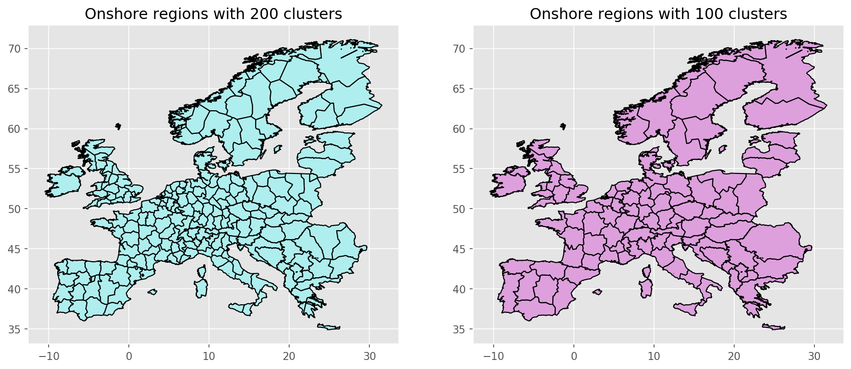
resources/regions_offshore_elec_s{simpl}_{clusters}.geojson: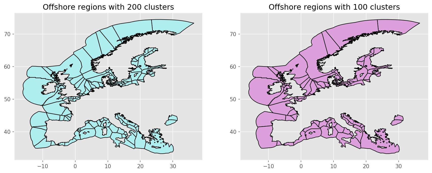
resources/busmap_elec_s{simpl}_{clusters}.csv: Mapping of buses fromnetworks/elec_s{simpl}.nctonetworks/elec_s{simpl}_{clusters}.nc;resources/linemap_elec_s{simpl}_{clusters}.csv: Mapping of lines fromnetworks/elec_s{simpl}.nctonetworks/elec_s{simpl}_{clusters}.nc;networks/elec_s{simpl}_{clusters}.nc: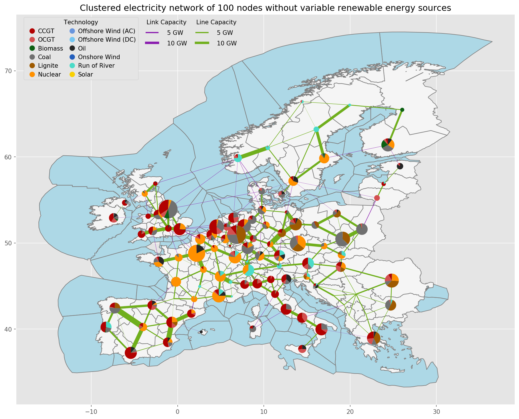
Description#
Note
Why is clustering used both in simplify_network and cluster_network ?
Consider for example a network
networks/elec_s100_50.ncin whichsimplify_networkclusters the network to 100 buses and in a second stepcluster_network`reduces it down to 50 buses.In preliminary tests, it turns out, that the principal effect of changing spatial resolution is actually only partially due to the transmission network. It is more important to differentiate between wind generators with higher capacity factors from those with lower capacity factors, i.e. to have a higher spatial resolution in the renewable generation than in the number of buses.
The two-step clustering allows to study this effect by looking at networks like
networks/elec_s100_50m.nc. Note the additionalmin the{cluster}wildcard. So in the example network there are still up to 100 different wind generators.In combination these two features allow you to study the spatial resolution of the transmission network separately from the spatial resolution of renewable generators.
Is it possible to run the model without the simplify_network rule?
No, the network clustering methods in the PyPSA module pypsa.clustering.spatial do not work reliably with multiple voltage levels and transformers.
Tip
The rule cluster_all_networks runs
for all scenario s in the configuration file
the rule cluster_network.
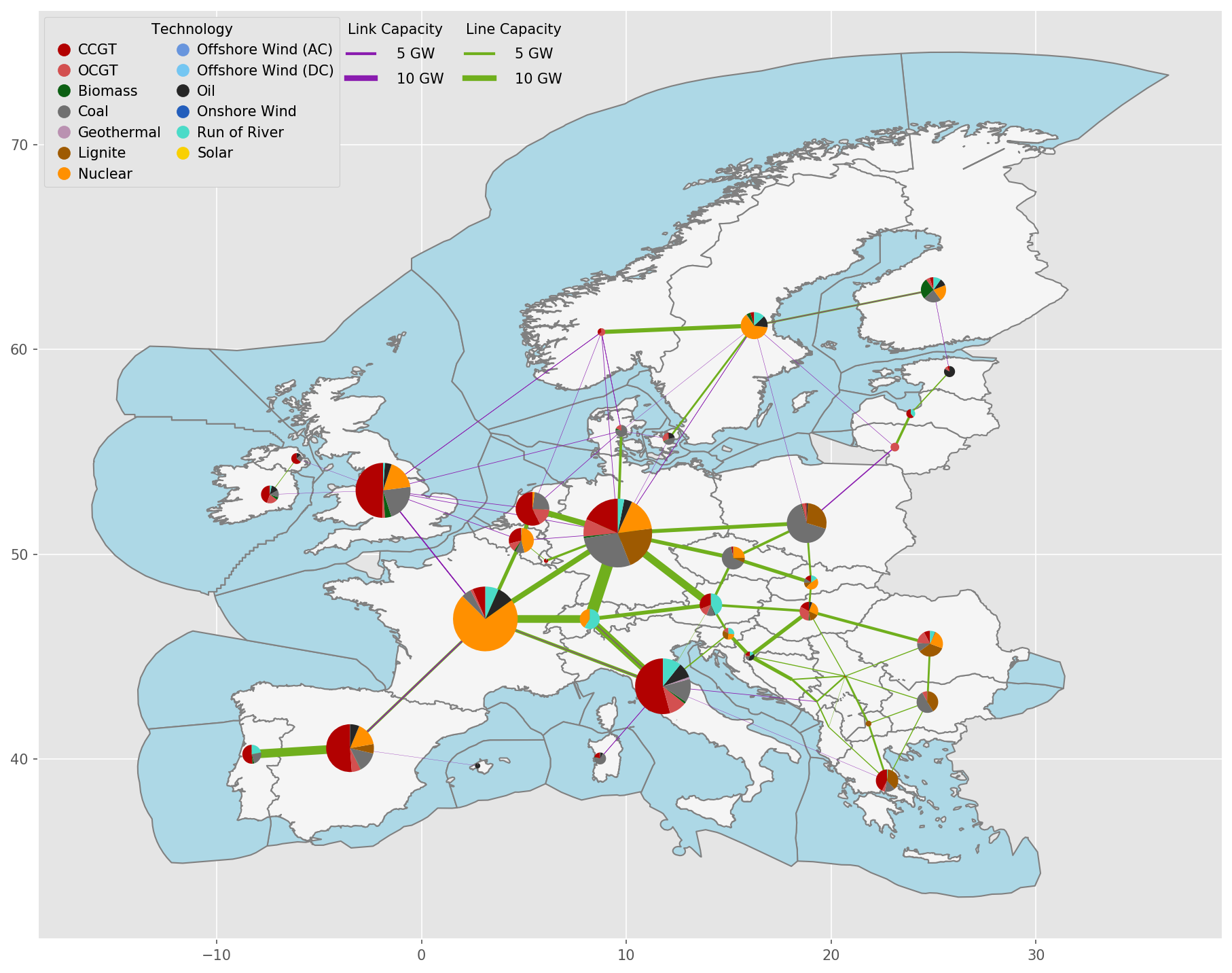
Exemplary unsolved network clustered to 512 nodes:
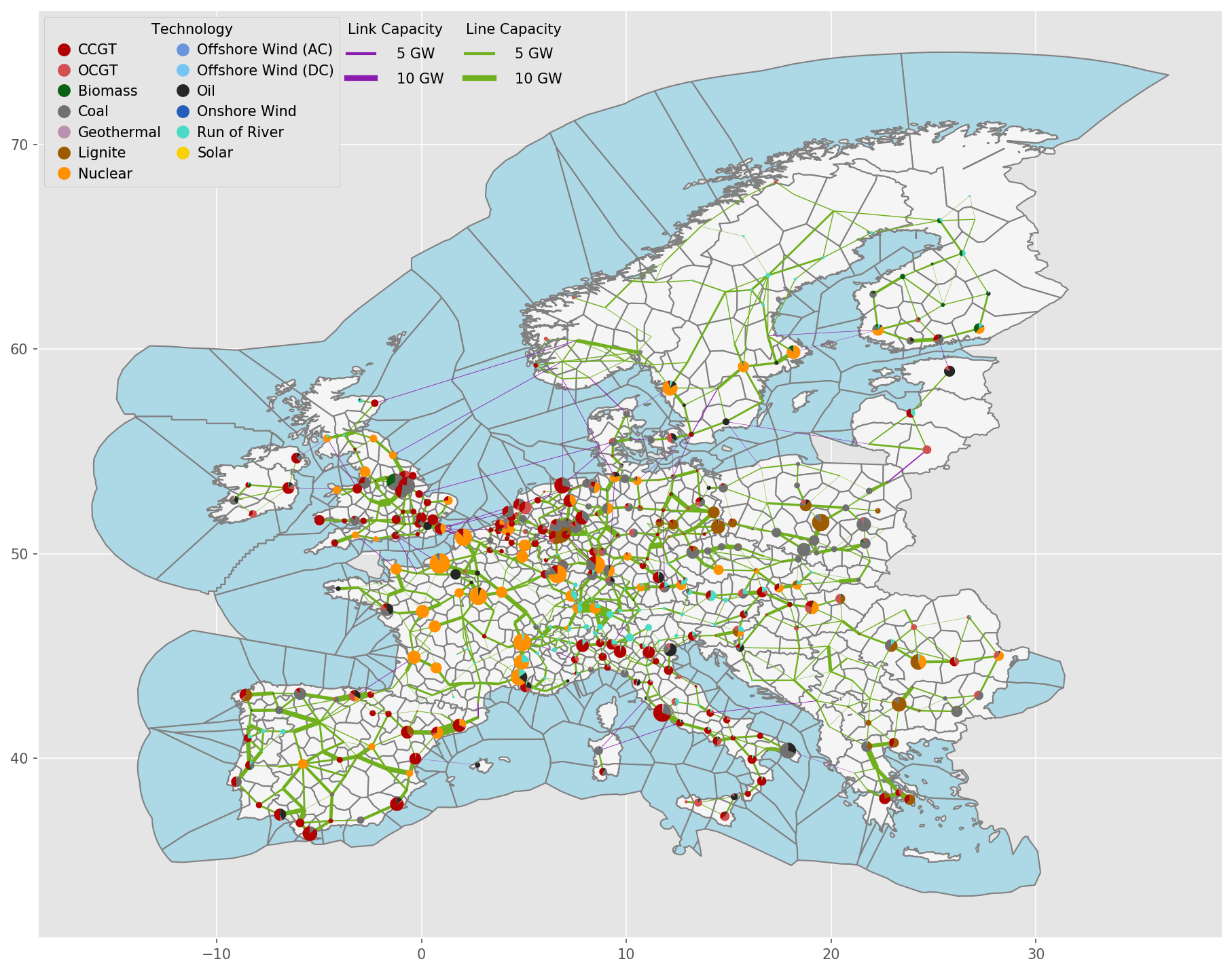
Exemplary unsolved network clustered to 256 nodes:

Exemplary unsolved network clustered to 128 nodes:
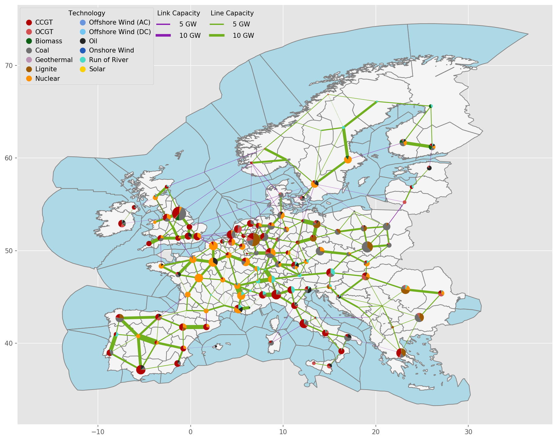
Exemplary unsolved network clustered to 37 nodes:
- cluster_network.distribute_clusters(inputs, build_shape_options, country_list, distribution_cluster, n, n_clusters, focus_weights=None, solver_name=None)#
Determine the number of clusters per country.
build_osm_network#
- build_osm_network.add_buses_to_empty_countries(country_list, fp_country_shapes, buses)#
Function to add a bus for countries missing substation data.
- build_osm_network.connect_stations_same_station_id(lines, buses)#
Function to create fake links between substations with the same substation_id.
- build_osm_network.fix_overpassing_lines(lines, buses, distance_crs, tol=1)#
Function to avoid buses overpassing lines with no connection when the bus is within a given tolerance from the line.
- Parameters:
lines (GeoDataFrame) – Geodataframe of lines
buses (GeoDataFrame) – Geodataframe of substations
tol (float) – Tolerance in meters of the distance between the substation and the line below which the line will be split
- build_osm_network.force_ac_lines(df, col='tag_frequency')#
Function that forces all PyPSA lines to be AC lines.
A network can contain AC and DC power lines that are modelled as PyPSA “Line” component. When DC lines are available, their power flow can be controlled by their converter. When it is artificially converted into AC, this feature is lost. However, for debugging and preliminary analysis, it can be useful to bypass problems.
- build_osm_network.get_ac_frequency(df, fr_col='tag_frequency')#
# Function to define a default frequency value.
Attempts to find the most usual non-zero frequency across the dataframe; 50 Hz is assumed as a back-up value
- build_osm_network.get_converters(buses, lines)#
Function to create fake converter lines that connect buses of the same station_id of different polarities.
- build_osm_network.get_transformers(buses, lines)#
Function to create fake transformer lines that connect buses of the same station_id at different voltage.
- build_osm_network.merge_stations_lines_by_station_id_and_voltage(lines, buses, geo_crs, distance_crs, tol=2000)#
Function to merge close stations and adapt the line datasets to adhere to the merged dataset.
- build_osm_network.merge_stations_same_station_id(buses, delta_lon=0.001, delta_lat=0.001, precision=4)#
Function to merge buses with same voltage and station_id This function iterates over all substation ids and creates a bus_id for every substation and voltage level.
Therefore, a substation with multiple voltage levels is represented with different buses, one per voltage level
- build_osm_network.set_lines_ids(lines, buses, distance_crs)#
Function to set line buses ids to the closest bus in the list.
- build_osm_network.set_lv_substations(buses)#
Function to set what nodes are lv, thereby setting substation_lv The current methodology is to set lv nodes to buses where multiple voltage level are found, hence when the station_id is duplicated.
- build_osm_network.set_substations_ids(buses, distance_crs, tol=2000)#
Function to set substations ids to buses, accounting for location tolerance.
The algorithm is as follows:
initialize all substation ids to -1
if the current substation has been already visited [substation_id < 0], then skip the calculation
- otherwise:
identify the substations within the specified tolerance (tol)
when all the substations in tolerance have substation_id < 0, then specify a new substation_id
otherwise, if one of the substation in tolerance has a substation_id >= 0, then set that substation_id to all the others; in case of multiple substations with substation_ids >= 0, the first value is picked for all
clean_osm_data#
- clean_osm_data.clean_cables(df)#
Function to clean the raw cables column: manual fixing and drop undesired values
- clean_osm_data.clean_circuits(df)#
Function to clean the raw circuits column: manual fixing and clean nan values
- clean_osm_data.clean_frequency(df, default_frequency='50')#
Function to clean raw frequency column: manual fixing and fill nan values
- clean_osm_data.clean_voltage(df)#
Function to clean the raw voltage column: manual fixing and drop nan values
- clean_osm_data.create_extended_country_shapes(country_shapes, offshore_shapes, tolerance=0.01)#
Obtain the extended country shape by merging on- and off-shore shapes.
- clean_osm_data.explode_rows(df, cols)#
Function that explodes the rows as specified in cols, including warning alerts for unexpected values.
Example
row 1: [50,50], [33000, 110000]
after explode_rows applied on the two columns becomes row 1: 50, 33000 row 2: 50, 110000
- clean_osm_data.fill_circuits(df)#
This function fills the rows circuits column so that the size of each list element matches the size of the list in the frequency column.
Multiple procedure are adopted:
In the rows of circuits where the number of elements matches the number of the frequency column, nothing is done
Where the number of elements in the cables column match the ones in the frequency column, then the values of cables are used.
Where the number of elements in cables exceed those in frequency, the cables elements are downscaled and the last values of cables are summed. Let’s assume that cables is [3,3,3] but frequency is [50,50]. With this procedures, cables is treated as [3,6] and used for calculating the circuits
Where the number in cables has an unique number, e.g. [‘6’], but frequency does not, e.g. [‘50’, ‘50’], then distribute the cables proportionally across the values. Note: the distribution accounts for the frequency type; when the frequency is 50 or 60, then a circuit requires 3 cables, when DC (0 frequency) is used, a circuit requires 2 cables.
Where no information of cables or circuits is available, a circuit is assumed for every frequency entry.
- clean_osm_data.filter_circuits(df, min_value_circuit=0.1)#
Filters df to contain only lines with circuit value above min_value_circuit.
- clean_osm_data.filter_frequency(df, accepted_values=[50, 60, 0], threshold=0.1)#
Filters df to contain only lines with frequency with accepted_values.
- clean_osm_data.filter_voltage(df, threshold_voltage=35000)#
Filters df to contain only lines with voltage above threshold_voltage.
- clean_osm_data.finalize_lines_type(df_lines)#
This function is aimed at finalizing the type of the columns of the dataframe.
- clean_osm_data.finalize_substation_types(df_all_substations)#
Specify bus_id and voltage columns as integer.
- clean_osm_data.find_first_overlap(geom, country_geoms, default_name)#
Return the first index whose shape intersects the geometry.
- clean_osm_data.integrate_lines_df(df_all_lines, distance_crs)#
Function to add underground, under_construction, frequency and circuits.
- clean_osm_data.load_network_data(network_asset, data_options)#
Function to check if OSM or custom data should be considered.
The network_asset should be a string named “lines”, “cables” or “substations”.
- clean_osm_data.prepare_generators_df(df_all_generators)#
Prepare the dataframe for generators.
- clean_osm_data.prepare_lines_df(df_lines)#
This function prepares the dataframe for lines and cables.
- Parameters:
df_lines (dataframe) – Raw lines or cables dataframe as downloaded from OpenStreetMap
- clean_osm_data.prepare_substation_df(df_all_substations)#
Prepare raw substations dataframe to the structure compatible with PyPSA- Eur.
- Parameters:
df_all_substations (dataframe) – Raw substations dataframe as downloaded from OpenStreetMap
- clean_osm_data.set_countryname_by_shape(df, ext_country_shapes, exclude_external=True, col_country='country')#
Set the country name by the name shape
- clean_osm_data.set_name_by_closestcity(df_all_generators, colname='name')#
Function to set the name column equal to the name of the closest city.
- clean_osm_data.set_unique_id(df, col)#
Create unique id’s, where id is specified by the column “col” The steps below create unique bus id’s without losing the original OSM bus_id.
Unique bus_id are created by simply adding -1,-2,-3 to the original bus_id Every unique id gets a -1 If a bus_id exist i.e. three times it it will the counted by cumcount -1,-2,-3 making the id unique
- Parameters:
df (dataframe) – Dataframe considered for the analysis
col (str) – Column name for the analyses; examples: “bus_id” for substations or “line_id” for lines
- clean_osm_data.split_and_match_voltage_frequency_size(df)#
Function to match the length of the columns in subset by duplicating the last value in the column.
The function does as follows:
First, it splits voltage and frequency columns by semicolon For example, the following lines row 1: ‘50’, ‘220000 row 2: ‘50;50;50’, ‘220000;380000’
become: row 1: [‘50’], [‘220000’] row 2: [‘50’,’50’,’50’], [‘220000’,’380000’]
Then, it harmonize each row to match the length of the lists by filling the missing values with the last elements of each list. In agreement to the example of before, after the cleaning:
row 1: [‘50’], [‘220000’] row 2: [‘50’,’50’,’50’], [‘220000’,’380000’,’380000’]
- clean_osm_data.split_cells(df, cols=['voltage'])#
Split semicolon separated cells i.e. [66000;220000] and create new identical rows.
- Parameters:
df (dataframe) – Dataframe under analysis
cols (list) – List of target columns over which to perform the analysis
Example
Original data: row 1: ‘66000;220000’, ‘50’
After applying split_cells(): row 1, ‘66000’, ‘50’ row 2, ‘220000’, ‘50’
download_osm_data#
Python interface to download OpenStreetMap data Documented at pypsa-meets-earth/earth-osm
Relevant Settings#
None # multiprocessing & infrastructure selection can be an option in future
Inputs#
None
Outputs#
data/osm/pbf: Raw OpenStreetMap data as .pbf files per countrydata/osm/power: Filtered power data as .json files per countrydata/osm/out: Prepared power data as .geojson and .csv files per countryresources/osm/raw: Prepared and per type (e.g. cable/lines) aggregated power data as .geojson and .csv files
- download_osm_data.convert_iso_to_geofk(iso_code, iso_coding=True, convert_dict={'AE': 'QA-AE-OM-BH-KW', 'AG': 'central-america', 'AS': 'american-oceania', 'AW': 'central-america', 'AX': 'finland', 'BB': 'central-america', 'BH': 'QA-AE-OM-BH-KW', 'BM': 'north-america', 'BN': 'MY', 'BS': 'bahamas', 'CP': 'ile-de-clipperton', 'CU': 'cuba', 'CW': 'central-america', 'DM': 'central-america', 'DO': 'haiti-and-domrep', 'EH': 'MA', 'FK': 'south-america', 'GD': 'central-america', 'GF': 'south-america', 'GG': 'guernsey-jersey', 'GM': 'SN-GM', 'GP': 'guadeloupe', 'GU': 'american-oceania', 'HK': 'china', 'HT': 'haiti-and-domrep', 'IC': 'canary-islands', 'IL': 'PS-IL', 'IM': 'isle-of-man', 'JE': 'guernsey-jersey', 'JM': 'jamaica', 'KM': 'comores', 'KN': 'central-america', 'KW': 'QA-AE-OM-BH-KW', 'KY': 'central-america', 'LC': 'central-america', 'MH': 'marshall-islands', 'MO': 'china', 'MP': 'american-oceania', 'NF': 'AU', 'OM': 'QA-AE-OM-BH-KW', 'PA': 'panama', 'PF': 'polynesie-francaise', 'PN': 'pitcairn-islands', 'PS': 'PS-IL', 'QA': 'QA-AE-OM-BH-KW', 'RE': 'reunion', 'SA': 'QA-AE-OM-BH-KW', 'SG': 'MY', 'SM': 'IT', 'SN': 'SN-GM', 'SX': 'central-america', 'TC': 'central-america', 'TK': 'tokelau', 'TT': 'central-america', 'VA': 'IT', 'VC': 'central-america', 'VU': 'vanuatu', 'WF': 'wallis-et-futuna', 'XK': 'RS-KM', 'YT': 'mayotte'})#
Function to convert the iso code name of a country into the corresponding geofabrik In Geofabrik, some countries are aggregated, thus if a single country is requested, then all the agglomeration shall be downloaded For example, Senegal (SN) and Gambia (GM) cannot be found alone in geofabrik, but they can be downloaded as a whole SNGM.
The conversion directory, initialized to iso_to_geofk_dict is used to perform such conversion When a two-letter code country is found in convert_dict, and iso_coding is enabled, then that two-letter code is converted into the corresponding value of the dictionary
- download_osm_data.country_list_to_geofk(country_list)#
Convert the requested country list into geofk norm.
- Parameters:
input (str) – Any two-letter country name or aggregation of countries given in the regions config file Country name duplications won’t distort the result. Examples are: [“NG”,”ZA”], downloading osm data for Nigeria and South Africa [“SNGM”], downloading data for Senegal&Gambia shape [“NG”,”ZA”,”NG”], won’t distort result.
- Returns:
full_codes_list – Example [“NG”,”ZA”]
- Return type:
simplify_network#
make_statistics#
Create statistics for a given scenario run.
This script contains functions to create statistics of the workflow for the current execution
Relevant statistics that are created are:
For clean_osm_data and download_osm_data, the number of elements, length of the lines and length of dc lines are stored
For build_shapes, the surface, total GDP, total population and number of shapes are collected
For build_renewable_profiles, total available potential and average production are collected
For network rules (base_network, add_electricity, simplify_network and solve_network), length of lines, number of buses and total installed capacity by generation technology
Execution time for the rules, when benchmark is available
Outputs#
This rule creates a dataframe containing in the columns the relevant statistics for the current run.
- make_statistics.add_computational_stats(df, snakemake, column_name=None)#
Add the major computational information of a given rule into the existing dataframe.
- make_statistics.aggregate_computational_stats(name, dict_dfs)#
Function to aggregate the total computational statistics of the rules.
- make_statistics.calculate_stats(scenario_config, renewable_config, renewable_carriers_config, metric_crs='EPSG:3857', area_crs='ESRI:54009')#
Function to collect all statistics
- make_statistics.collect_basic_osm_stats(path, rulename, header)#
Collect basic statistics on OSM data: number of items
- make_statistics.collect_bus_regions_stats(bus_region_rule='build_bus_regions')#
Collect statistics on bus regions.
number of onshore regions
number of offshore regions
- make_statistics.collect_clean_osm_stats(rulename='clean_osm_data', metric_crs='EPSG:3857')#
Collect statistics on OSM data; used for clean OSM data.
- make_statistics.collect_network_osm_stats(path, rulename, header, metric_crs='EPSG:3857')#
Collect statistics on OSM network data: - number of items - length of the stored shapes - length of objects with tag_frequency == 0 (DC elements)
- make_statistics.collect_network_stats(network_rule, scenario_config)#
Collect statistics on pypsa networks: - installed capacity by carrier - lines total length (accounting for parallel lines) - lines total capacity
- make_statistics.collect_only_computational(rulename)#
Rule to create only computational statistics of rule rulename.
- make_statistics.collect_osm_stats(rulename, **kwargs)#
Collect statistics on OSM data.
When lines and cables are considered, then network-related statistics are collected (collect_network_osm_stats), otherwise basic statistics are (collect_basic_osm_stats)
- make_statistics.collect_raw_osm_stats(rulename='download_osm_data', metric_crs='EPSG:3857')#
Collect basic statistics on OSM data; used for raw OSM data.
- make_statistics.collect_renewable_stats(rulename, technology)#
Collect statistics on the renewable time series generated by the workflow: - potential - average production by plant (hydro) or bus (other RES)
- make_statistics.collect_shape_stats(rulename='build_shapes', area_crs='ESRI:54009')#
Collect statistics on the shapes created by the workflow: - area - number of gadm shapes - Percentage of shapes having country flag matching the gadm file - total population - total gdp
- make_statistics.collect_snakemake_stats(name, dict_dfs, renewable_config, renewable_carriers_config)#
Collect statistics on what rules have been successful.
- make_statistics.generate_scenario_by_country(path_base, country_list, out_dir='configs/scenarios', pre='config.')#
Utility function to create copies of a standard yaml file available in path_base for every country in country_list. Copies are saved into the output directory out_dir.
Note: - the clusters are automatically modified for selected countries with limited data - for landlocked countries, offwind technologies are removed (solar, onwind and hydro are forced)
monte_carlo#
Prepares network files with monte-carlo parameter sweeps for solving process.
Relevant Settings#
monte_carlo:
options:
    add_to_snakefile: false # When set to true, enables Monte Carlo sampling
    samples: 9 # number of optimizations. Note that number of samples when using scipy has to be the square of a prime number
    sampling_strategy: "chaospy"  # "pydoe2", "chaospy", "scipy", packages that are supported
    seed: 42 # set seedling for reproducibilty
uncertainties:
    loads_t.p_set:
      type: uniform
      args: [0, 1]
    generators_t.p_max_pu.loc[:, n.generators.carrier == "onwind"]:
      type: lognormal
      args: [1.5]
    generators_t.p_max_pu.loc[:, n.generators.carrier == "solar"]:
      type: beta
      args: [0.5, 2]
See also
Documentation of the configuration file config.yaml at monte_carlo
Inputs#
networks/elec_s_10_ec_lcopt_Co2L-24H.nc
Outputs#
networks/elec_s_10_ec_lcopt_Co2L-24H_{unc}.nc
- e.g. networks/elec_s_10_ec_lcopt_Co2L-24H_m0.nc
networks/elec_s_10_ec_lcopt_Co2L-24H_m1.nc …
Description#
PyPSA-Earth is deterministic which means that a set of inputs give a set of outputs. Parameter sweeps can help to explore the uncertainty of the outputs cause by parameter changes. Many are familiar with the classical “sensitivity analysis” that can be applied by varying the input of only one feature, while exploring its outputs changes. Here implemented is a “global sensitivity analysis” that can help to explore the multi-dimensional uncertainty space when more than one feature are changed at the same time.
To do so, the scripts is separated in two building blocks: One creates the experimental design, the other, modifies and outputs the network file. Building the experimental design is currently supported by the packages pyDOE2, chaospy and scipy. This should give users the freedom to explore alternative approaches. The orthogonal latin hypercube sampling is thereby found as most performant, hence, implemented here. Sampling the multi-dimensional uncertainty space is relatively easy. It only requires two things: The number of samples (defines the number of total networks to be optimized) and features (pypsa network object e.g loads_t.p_set or generators_t.p_max_pu). This results in an experimental design of the dimension (samples X features).
The experimental design lh (dimension: sample X features) is used to modify the PyPSA networks. Thereby, this script creates samples x amount of networks. The iterators comes from the wildcard {unc}, which is described in the config.yaml and created in the Snakefile as a range from 0 to (total number of) SAMPLES.
- monte_carlo.monte_carlo_sampling_chaospy(N_FEATURES: int, SAMPLES: int, uncertainties_values: dict, seed: int, rule: str = 'latin_hypercube') ndarray#
Creates Latin Hypercube Sample (LHS) implementation from chaospy.
Documentation on Chaospy: clicumu/pyDOE2 (fixes latin_cube errors) Documentation on Chaospy latin-hyper cube (quasi-Monte Carlo method): https://chaospy.readthedocs.io/en/master/user_guide/fundamentals/quasi_random_samples.html#Quasi-random-samples
- monte_carlo.monte_carlo_sampling_pydoe2(N_FEATURES: int, SAMPLES: int, uncertainties_values: dict, random_state: int, criterion: str = None, iteration: int = None, correlation_matrix: ndarray = None) ndarray#
Creates Latin Hypercube Sample (LHS) implementation from PyDOE2 with various options. Additionally, all “corners” are simulated.
Adapted from Disspaset: energy-modelling-toolkit/Dispa-SET Documentation on PyDOE2: clicumu/pyDOE2 (fixes latin_cube errors)
- monte_carlo.monte_carlo_sampling_scipy(N_FEATURES: int, SAMPLES: int, uncertainties_values: dict, seed: int, strength: int = 2, optimization: str = None) ndarray#
Creates Latin Hypercube Sample (LHS) implementation from SciPy with various options:
Center the point within the multi-dimensional grid, centered=True
Optimization scheme, optimization=”random-cd”
Strength=1, classical LHS
Strength=2, performant orthogonal LHS, requires the sample to be square of a prime e.g. sq(11)=121
Options could be combined to produce an optimized centered orthogonal array based LHS. After optimization, the result would not be guaranteed to be of strength 2.
Documentation for Quasi-Monte Carlo approaches: https://docs.scipy.org/doc/scipy/reference/stats.qmc.html Documentation for Latin Hypercube: https://docs.scipy.org/doc/scipy/reference/generated/scipy.stats.qmc.LatinHypercube.html#scipy.stats.qmc.LatinHypercube Orthogonal LHS is better than basic LHS: scipy/scipy#files, https://en.wikipedia.org/wiki/Latin_hypercube_sampling
- monte_carlo.rescale_distribution(latin_hypercube: ndarray, uncertainties_values: dict) ndarray#
Rescales a Latin hypercube sampling (LHS) using specified distribution parameters. More information on the distributions can be found here https://docs.scipy.org/doc/scipy/reference/stats.html
Parameters:
latin_hypercube (np.array): The Latin hypercube sampling to be rescaled.
uncertainties_values (list): List of dictionaries containing distribution information.
Each dictionary should have ‘type’ key specifying the distribution type and ‘args’ key containing parameters specific to the chosen distribution.
Returns:
np.array: Rescaled Latin hypercube sampling with values in the range [0, 1].
Supported Distributions:
“uniform”: Rescaled to the specified lower and upper bounds.
“normal”: Rescaled using the inverse of the normal distribution function with specified mean and std.
“lognormal”: Rescaled using the inverse of the log-normal distribution function with specified mean and std.
“triangle”: Rescaled using the inverse of the triangular distribution function with mean calculated from given parameters.
“beta”: Rescaled using the inverse of the beta distribution function with specified shape parameters.
“gamma”: Rescaled using the inverse of the gamma distribution function with specified shape and scale parameters.
Note:
The function supports rescaling for uniform, normal, lognormal, triangle, beta, and gamma distributions.
The rescaled samples will have values in the range [0, 1].
- monte_carlo.validate_parameters(sampling_strategy: str, samples: int, uncertainties_values: dict) None#
Validates the parameters for a given probability distribution. Inputs from user through the config file needs to be validated before proceeding to perform monte-carlo simulations.
Parameters:
- sampling_strategy: str
The chosen sampling strategy from chaospy, scipy and pydoe2
- samples: int
The number of samples to generate for the simulation
- distribution: str
The name of the probability distribution.
- distribution_params: list
The parameters associated with the probability distribution.
Raises:
ValueError: If the parameters are invalid for the specified distribution.