API Reference (automated)

_helpers

_helpers.configure_logging(snakemake, skip_handlers=False)

Configure the basic behaviour for the logging module.

Note: Must only be called once from the __main__ section of a script.

The setup includes printing log messages to STDERR and to a log file defined by either (in priority order): snakemake.log.python, snakemake.log[0] or “logs/{rulename}.log”. Additional keywords from logging.basicConfig are accepted via the snakemake configuration file under snakemake.config.logging.

Parameters:

• snakemake (snakemake object) – Your snakemake object containing a snakemake.config and snakemake.log.

• skip_handlers (True | False (default)) – Do (not) skip the default handlers created for redirecting output to STDERR and file.

_helpers.country_name_2_two_digits(country_name)

Convert full country name to 2-digit country code.

Parameters:

country_name (str) – country name

Returns:

two_code_country – 2-digit country name

Return type:

str

_helpers.create_country_list(input, iso_coding=True)

Create a country list for defined regions in config_osm_data.py.

Parameters:

input (str) – Any two-letter country name, regional name, or continent given in config_osm_data.py Country name duplications won’t distort the result. Examples are: [“NG”,”ZA”], downloading osm data for Nigeria and South Africa [“africa”], downloading data for Africa [“NAR”], downloading data for the North African Power Pool [“TEST”], downloading data for a customized test set. [“NG”,”ZA”,”NG”], won’t distort result.

Returns:

full_codes_list – Example [“NG”,”ZA”]

Return type:

list

_helpers.getContinent(code)

Returns continent names that contains list of iso-code countries.

Parameters:

code (str) – List of two letter country ISO codes

Returns:

continent_list – List of continent names

Return type:

str

Example

from helpers import getContinent code = [“DE”, “GB”, “NG”, “ZA”] getContinent(code) >>> [“africa”, “europe”]

_helpers.get_aggregation_strategies(aggregation_strategies)

Default aggregation strategies that cannot be defined in .yaml format must be specified within the function, otherwise (when defaults are passed in the function’s definition) they get lost when custom values are specified in the config.

_helpers.get_last_commit_message()

Function to get the last Git commit message.

Returns:

result

Return type:

string

_helpers.load_network(import_name=None, custom_components=None)

Helper for importing a pypsa.Network with additional custom components.

Parameters:

• import_name (str) – As in pypsa.Network(import_name)

• custom_components (dict) –

  Dictionary listing custom components. For using snakemake.params.override_components"] in config.yaml define:

  override_components:
      ShadowPrice:
          component: ["shadow_prices","Shadow price for a global constraint.",np.nan]
          attributes:
          name: ["string","n/a","n/a","Unique name","Input (required)"]
          value: ["float","n/a",0.,"shadow value","Output"]
  

Return type:

pypsa.Network

_helpers.mock_snakemake(rulename, **wildcards)

This function is expected to be executed from the “scripts”-directory of ” the snakemake project. It returns a snakemake.script.Snakemake object, based on the Snakefile.

If a rule has wildcards, you have to specify them in **wildcards.

Parameters:

• rulename (str) – name of the rule for which the snakemake object should be generated

• **wildcards – keyword arguments fixing the wildcards. Only necessary if wildcards are needed.

_helpers.progress_retrieve(url, file, data=None, disable_progress=False, roundto=1.0)

Function to download data from a url with a progress bar progress in retrieving data.

Parameters:

• url (str) – Url to download data from

• file (str) – File where to save the output

• data (dict) – Data for the request (default None), when not none Post method is used

• disable_progress (bool) – When true, no progress bar is shown

• roundto (float) – (default 0) Precision used to report the progress e.g. 0.1 stands for 88.1, 10 stands for 90, 80

_helpers.read_csv_nafix(file, **kwargs)

Function to open a csv as pandas file and standardize the na value

_helpers.read_geojson(fn, cols=[], dtype=None, crs='EPSG:4326')

Function to read a geojson file fn. When the file is empty, then an empty GeoDataFrame is returned having columns cols, the specified crs and the columns specified by the dtype dictionary it not none.

Parameters:

fnstr

Path to the file to read

colslist

List of columns of the GeoDataFrame

dtypedict

Dictionary of the type of the object by column

crsstr

CRS of the GeoDataFrame

_helpers.read_osm_config(*args)

Read values from the osm_config.yaml file based on provided key arguments.

Parameters:

*args (str) – One or more key arguments corresponding to the values to retrieve from the config file. Typical arguments include “world_iso”, “continent_regions”, “iso_to_geofk_dict”, and “osm_clean_columns”.

Returns:

If a single key is provided, returns the corresponding value from the osm_config.yaml file. If multiple keys are provided, returns a tuple containing values corresponding to the provided keys.

Return type:

tuple or str or dict

Examples

>>> values = read_osm_config("key1", "key2")
>>> print(values)
('value1', 'value2')

>>> world_iso = read_osm_config("world_iso")
>>> print(world_iso)
{"Africa": {"DZ": "algeria", ...}, ...}

_helpers.sets_path_to_root(root_directory_name)

Search and sets path to the given root directory (root/path/file).

Parameters:

• root_directory_name (str) – Name of the root directory.

• n (int) – Number of folders the function will check upwards/root directed.

_helpers.three_2_two_digits_country(three_code_country)

Convert 3-digit to 2-digit country code:

Parameters:

three_code_country (str) – 3-digit country name

Returns:

two_code_country – 2-digit country name

Return type:

str

_helpers.two_2_three_digits_country(two_code_country)

Convert 2-digit to 3-digit country code:

Parameters:

two_code_country (str) – 2-digit country name

Returns:

three_code_country – 3-digit country name

Return type:

str

_helpers.two_digits_2_name_country(two_code_country, nocomma=False, remove_start_words=[])

Convert 2-digit country code to full name country:

Parameters:

• two_code_country (str) – 2-digit country name

• nocomma (bool (optional, default False)) – When true, country names with comma are extended to remove the comma. Example CD -> Congo, The Democratic Republic of -> The Democratic Republic of Congo

• remove_start_words (list (optional, default empty)) – When a sentence starts with any of the provided words, the beginning is removed. e.g. The Democratic Republic of Congo -> Democratic Republic of Congo (remove_start_words=[“The”])

Returns:

full_name – full country name

Return type:

str

add_electricity

Adds electrical generators, load and existing hydro storage units to a base network.

Relevant Settings

costs:
    year:
    version:
    rooftop_share:
    USD2013_to_EUR2013:
    dicountrate:
    emission_prices:

electricity:
    max_hours:
    marginal_cost:
    capital_cost:
    conventional_carriers:
    co2limit:
    extendable_carriers:
    include_renewable_capacities_from_OPSD:
    estimate_renewable_capacities_from_capacity_stats:

renewable:
    hydro:
        carriers:
        hydro_max_hours:
        hydro_max_hours_default:
        hydro_capital_cost:

lines:
    length_factor:

See also

Documentation of the configuration file config.yaml at costs, electricity, load_options, renewable, lines

Inputs

• resources/costs.csv: The database of cost assumptions for all included technologies for specific years from various sources; e.g. discount rate, lifetime, investment (CAPEX), fixed operation and maintenance (FOM), variable operation and maintenance (VOM), fuel costs, efficiency, carbon-dioxide intensity.

• data/bundle/hydro_capacities.csv: Hydropower plant store/discharge power capacities, energy storage capacity, and average hourly inflow by country. Not currently used!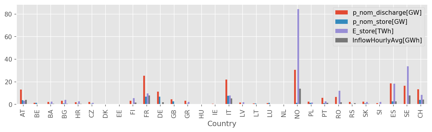

  

• data/geth2015_hydro_capacities.csv: alternative to capacities above; not currently used!

• resources/demand_profiles.csv: a csv file containing the demand profile associated with buses

• resources/shapes/gadm_shapes.geojson: confer Rule build_shapes

• resources/powerplants.csv: confer Rule build_powerplants

• resources/profile_{}.nc: all technologies in config["renewables"].keys(), confer Rule build_renewable_profiles

• networks/base.nc: confer Rule base_network

Outputs

• networks/elec.nc: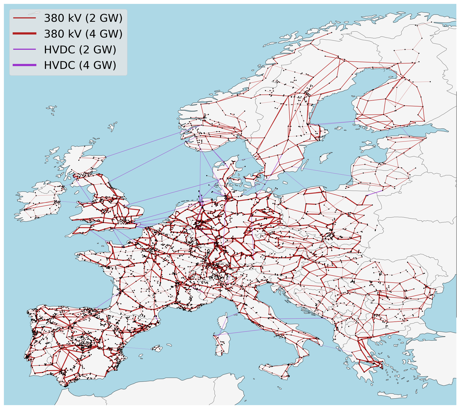

  

Description

The rule add_electricity ties all the different data inputs from the preceding rules together into a detailed PyPSA network that is stored in networks/elec.nc. It includes:

• today’s transmission topology and transfer capacities (in future, optionally including lines which are under construction according to the config settings lines: under_construction and links: under_construction),

• today’s thermal and hydro power generation capacities (for the technologies listed in the config setting electricity: conventional_carriers), and

• today’s load time-series (upsampled in a top-down approach according to population and gross domestic product)

It further adds extendable generators with zero capacity for

• photovoltaic, onshore and AC- as well as DC-connected offshore wind installations with today’s locational, hourly wind and solar capacity factors (but no current capacities),

• additional open- and combined-cycle gas turbines (if OCGT and/or CCGT is listed in the config setting electricity: extendable_carriers)

add_electricity.attach_load(n, demand_profiles)

Add load profiles to network buses.

Parameters:

• n (pypsa network)

• demand_profiles (str) – Path to csv file of elecric demand time series, e.g. “resources/demand_profiles.csv” Demand profile has snapshots as rows and bus names as columns.

Returns:

n – Now attached with load time series

Return type:

pypsa network

add_electricity.calculate_annuity(n, r)

Calculate the annuity factor for an asset with lifetime n years and discount rate of r, e.g. annuity(20, 0.05) * 20 = 1.6.

add_electricity.load_costs(tech_costs, config, elec_config, Nyears=1)

Set all asset costs and other parameters.

base_network

Creates the network topology from a OpenStreetMap.

Relevant Settings

snapshots:

countries:

electricity:
    voltages:

lines:
    types:
    s_max_pu:
    under_construction:

links:
    p_max_pu:
    p_nom_max:
    under_construction:

transformers:
    x:
    s_nom:
    type:

See also

Documentation of the configuration file config.yaml at snapshots, Top-level configuration, electricity, load_options, lines, links, transformers

Inputs

Outputs

• networks/base.nc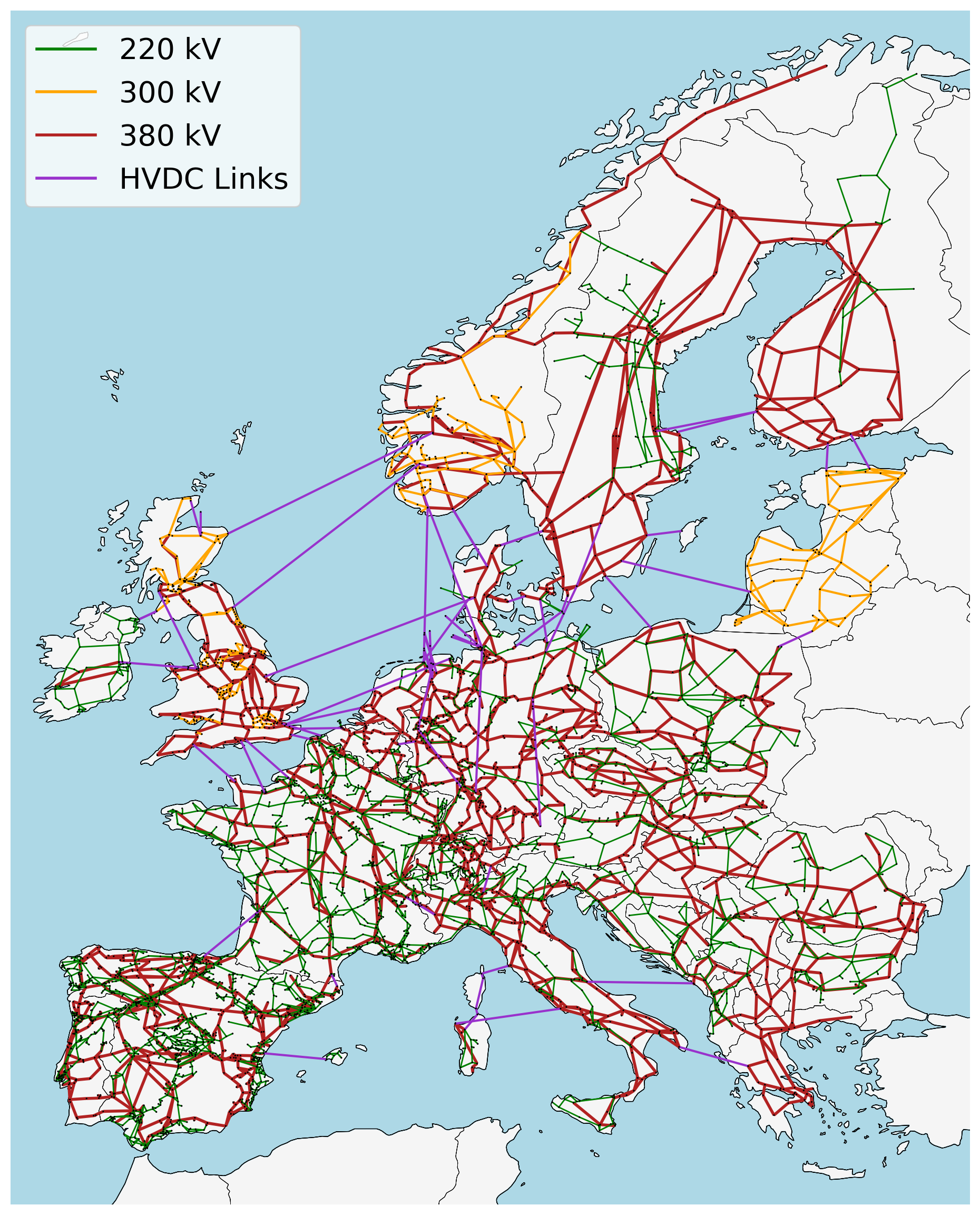

  

Description

build_bus_regions

Creates Voronoi shapes for each bus representing both onshore and offshore regions.

Relevant Settings

countries:

See also

Documentation of the configuration file config.yaml at Top-level configuration

Inputs

• resources/country_shapes.geojson: confer Rule build_shapes

• resources/offshore_shapes.geojson: confer Rule build_shapes

• networks/base.nc: confer Rule base_network

Outputs

• resources/regions_onshore.geojson: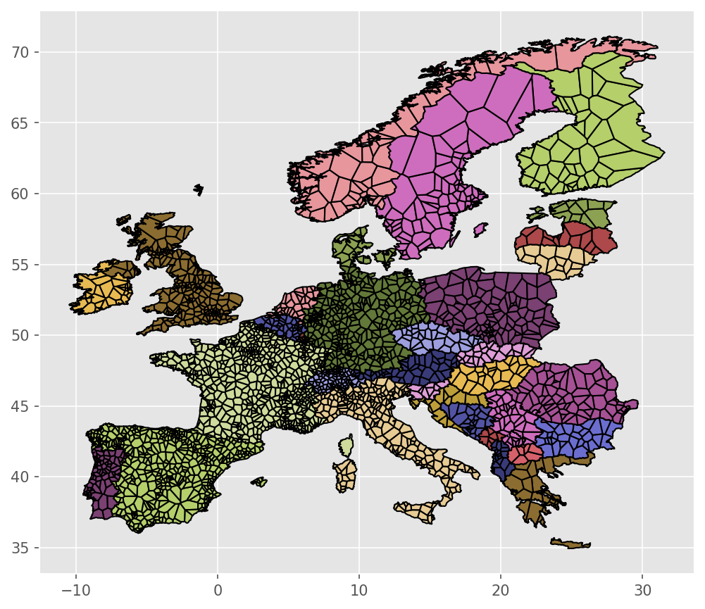

  

• resources/regions_offshore.geojson: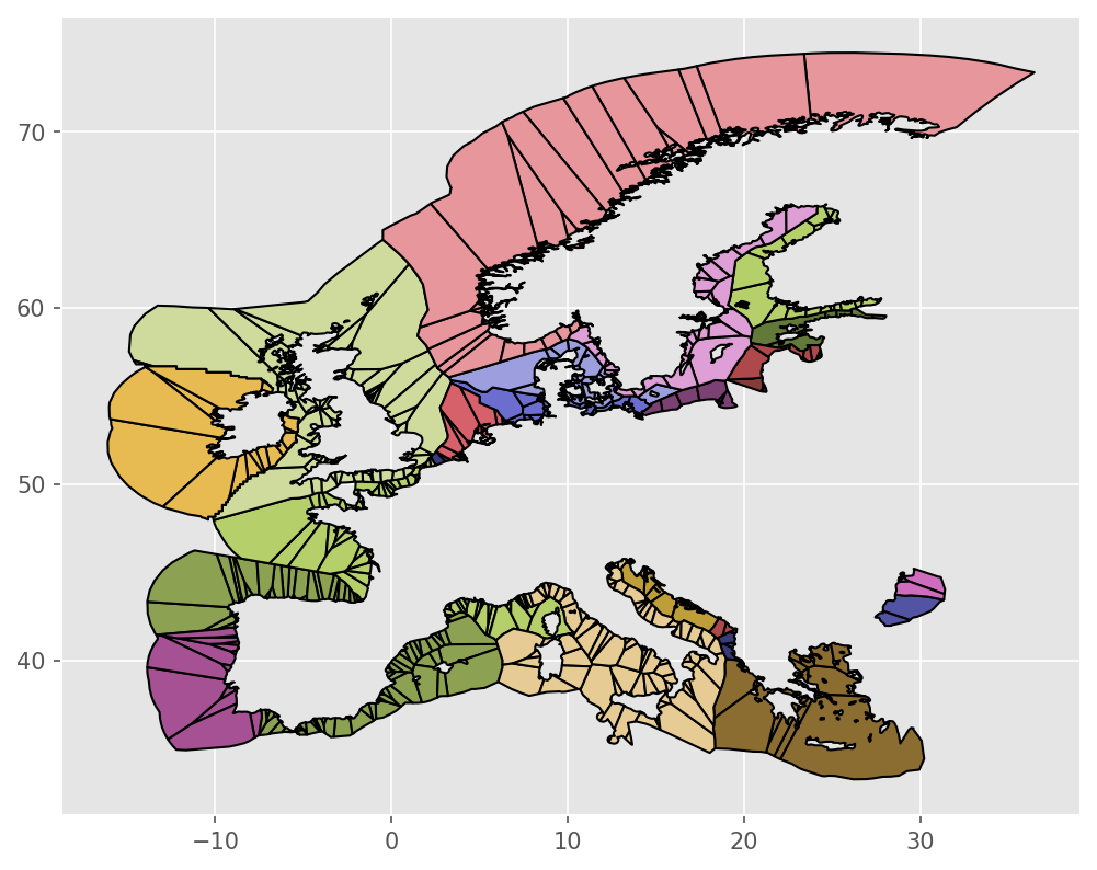

  

Description

build_bus_regions.custom_voronoi_partition_pts(points, outline, add_bounds_shape=True, multiplier=5)

Compute the polygons of a voronoi partition of points within the polygon outline

build_bus_regions.points

Type:

Nx2 - ndarray[dtype=float]

build_bus_regions.outline

Type:

Polygon

Returns:

polygons

Return type:

N - ndarray[dtype=Polygon|MultiPolygon]

build_cutout

Create cutouts with atlite.

For this rule to work you must have

• installed the Copernicus Climate Data Store cdsapi package (install with `pip`) and

• registered and setup your CDS API key as described on their website. The CDS API allows an automatic filedownload by executing this script

See also

For details on the weather data read the atlite documentation. If you need help specifically for creating cutouts the corresponding section in the atlite documentation should be helpful.

Relevant Settings

atlite:
    nprocesses:
    cutouts:
        {cutout}:

See also

Documentation of the configuration file config.yaml at atlite

Inputs

None

Outputs

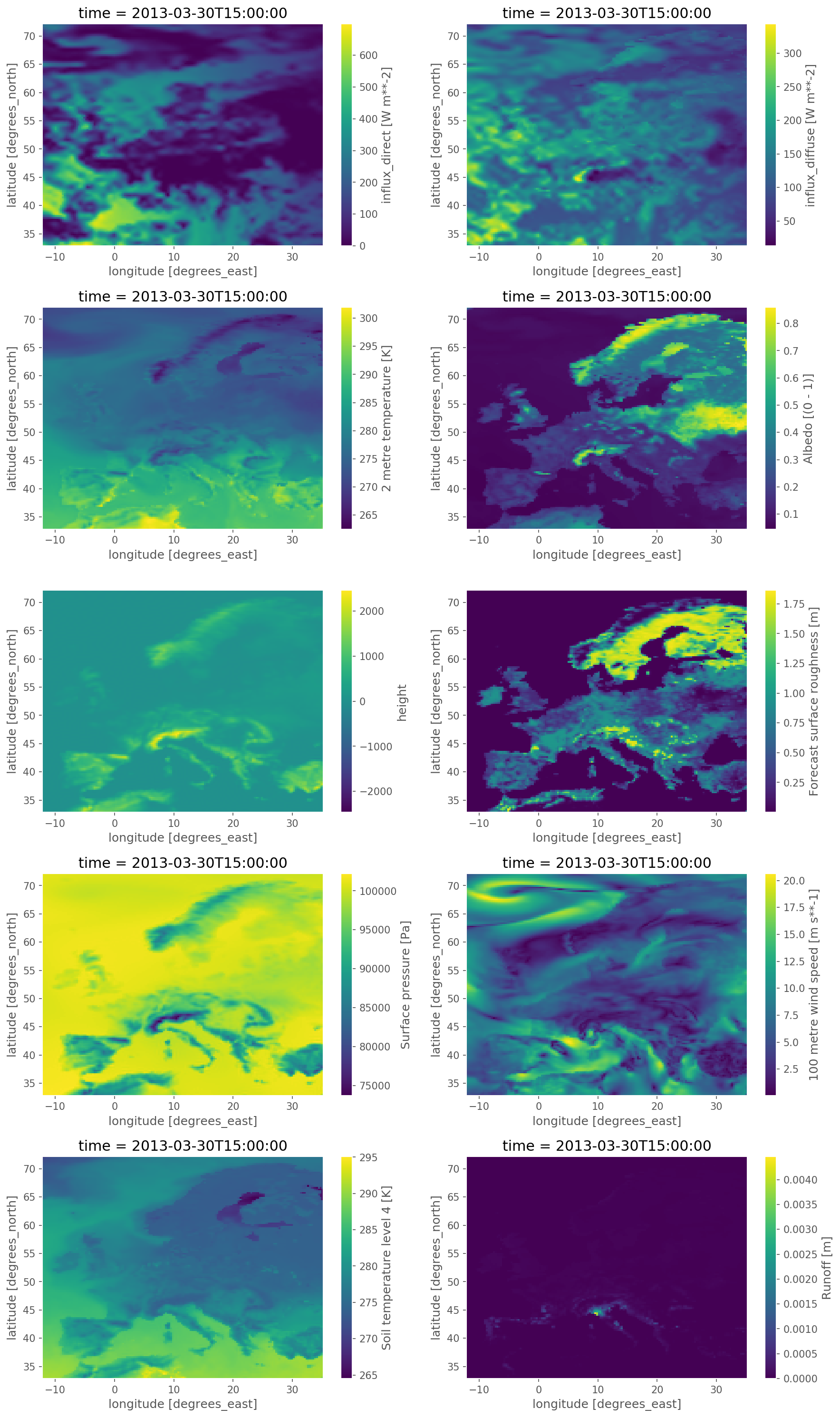
• cutouts/{cutout}: weather data from either the ERA5 reanalysis weather dataset or SARAH-2 satellite-based historic weather data with the following structure:

ERA5 cutout:

Field	Dimensions	Unit	Description
pressure	time, y, x	Pa	Surface pressure
temperature	time, y, x	K	Air temperature 2 meters above the surface.
soil temperature	time, y, x	K	Soil temperature between 1 meters and 3 meters depth (layer 4).
influx_toa	time, y, x	Wm**-2	Top of Earth’s atmosphere TOA incident solar radiation
influx_direct	time, y, x	Wm**-2	Total sky direct solar radiation at surface
runoff	time, y, x	m	Runoff (volume per area)
roughness	y, x	m	Forecast surface roughness (roughness length)
height	y, x	m	Surface elevation above sea level
albedo	time, y, x	–	Albedo measure of diffuse reflection of solar radiation. Calculated from relation between surface solar radiation downwards (Jm**-2) and surface net solar radiation (Jm**-2). Takes values between 0 and 1.
influx_diffuse	time, y, x	Wm**-2	Diffuse solar radiation at surface. Surface solar radiation downwards minus direct solar radiation.
wnd100m	time, y, x	ms**-1	Wind speeds at 100 meters (regardless of direction)

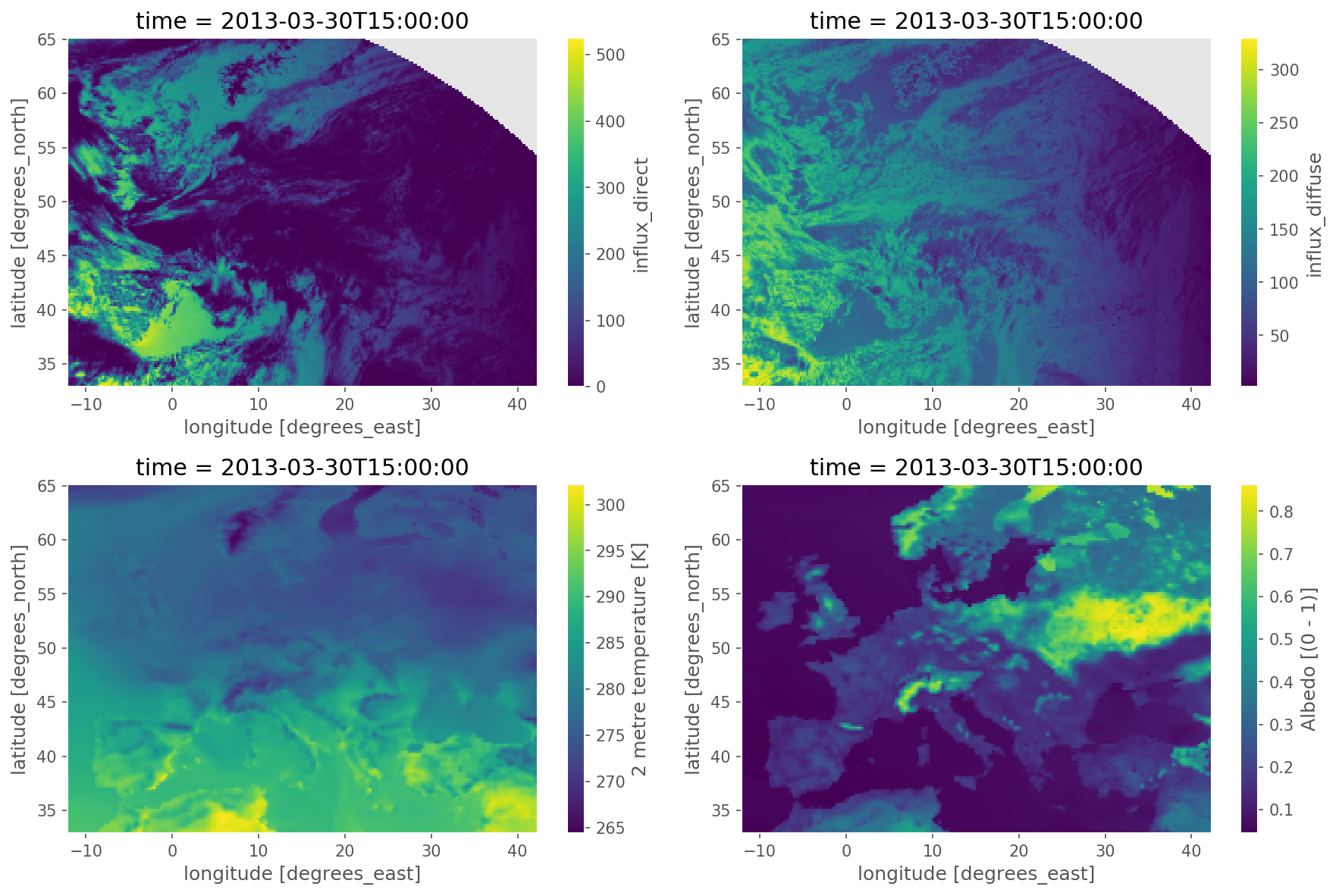
A SARAH-2 cutout can be used to amend the fields temperature, influx_toa, influx_direct, albedo, influx_diffuse of ERA5 using satellite-based radiation observations.

Description

build_demand_profiles

Creates electric demand profile csv.

Relevant Settings

load:
    scale:
    ssp:
    weather_year:
    prediction_year:
    region_load:

Inputs

• networks/base.nc: confer Rule base_network, a base PyPSA Network

• resources/bus_regions/regions_onshore.geojson: confer build_bus_regions

• load_data_paths: paths to load profiles, e.g. hourly country load profiles produced by GEGIS

• resources/shapes/gadm_shapes.geojson: confer Rule build_shapes, file containing the gadm shapes

Outputs

• resources/demand_profiles.csv: the content of the file is the electric demand profile associated to each bus. The file has the snapshots as rows and the buses of the network as columns.

Description

The rule build_demand creates load demand profiles in correspondence of the buses of the network. It creates the load paths for GEGIS outputs by combining the input parameters of the countries, weather year, prediction year, and SSP scenario. Then with a function that takes in the PyPSA network “base.nc”, region and gadm shape data, the countries of interest, a scale factor, and the snapshots, it returns a csv file called “demand_profiles.csv”, that allocates the load to the buses of the network according to GDP and population.

build_demand_profiles.build_demand_profiles(n, load_paths, regions, admin_shapes, countries, scale, start_date, end_date, out_path)

Create csv file of electric demand time series.

Parameters:

• n (pypsa network)

• load_paths (paths of the load files)

• regions (.geojson) – Contains bus_id of low voltage substations and bus region shapes (voronoi cells)

• admin_shapes (.geojson) – contains subregional gdp, population and shape data

• countries (list) – List of countries that is config input

• scale (float) – The scale factor is multiplied with the load (1.3 = 30% more load)

• start_date (parameter) – The start_date is the first hour of the first day of the snapshots

• end_date (parameter) – The end_date is the last hour of the last day of the snapshots

Returns:

demand_profiles.csv

Return type:

csv file containing the electric demand time series

build_demand_profiles.get_load_paths_gegis(ssp_parentfolder, config)

Create load paths for GEGIS outputs.

The paths are created automatically according to included country, weather year, prediction year and ssp scenario

Example

[“/data/ssp2-2.6/2030/era5_2013/Africa.nc”, “/data/ssp2-2.6/2030/era5_2013/Africa.nc”]

build_demand_profiles.shapes_to_shapes(orig, dest)

Adopted from vresutils.transfer.Shapes2Shapes()

build_natura_raster

Converts vectordata or known as shapefiles (i.e. used for geopandas/shapely) to our cutout rasters. The Protected Planet Data on protected areas is aggregated to all cutout regions.

Relevant Settings

renewable:
    {technology}:
        cutout:

See also

Documentation of the configuration file config.yaml at renewable

Inputs

• data/raw/protected_areas/WDPA_WDOECM_Aug2021_Public_AF_shp-points.shp: WDPA World Database for Protected Areas.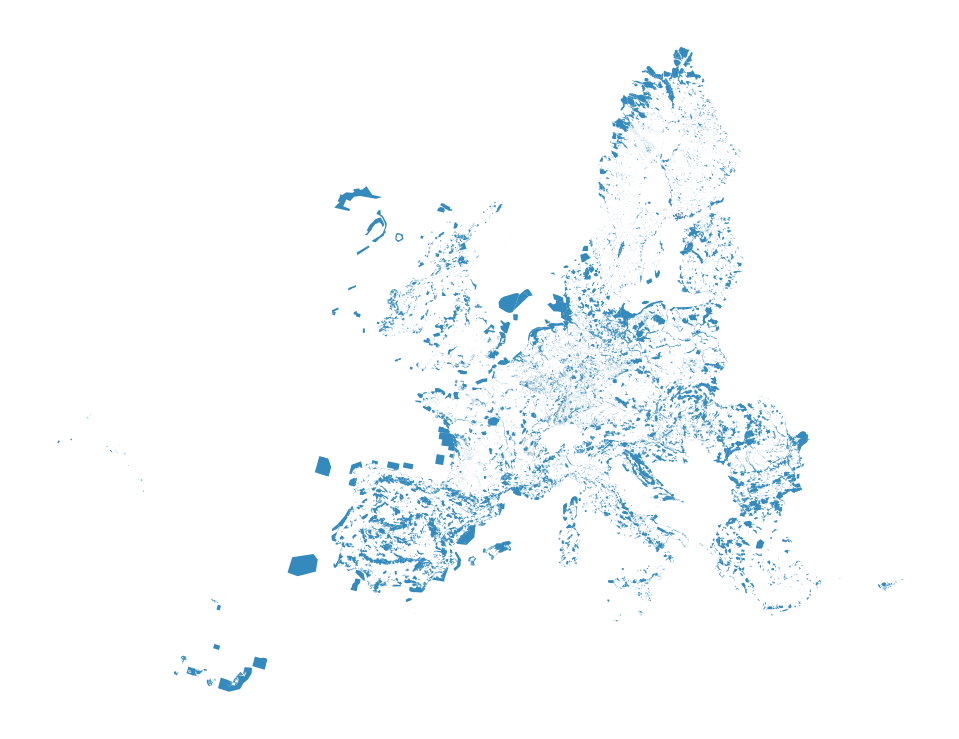

  

Outputs

• resources/natura.tiff: Rasterized version of Natura 2000 natural protection areas to reduce computation times.

  

Description

To operate the script you need all input files. The Snakefile describes what goes in and out. Make sure you didn’t skip one of these. Maybe not so obvious is the cutout input. An example is this africa-2013-era5.nc

Steps to retrieve the protected area data (as apparently no API is given for the WDPA data):

• 1. Download the WPDA Dataset: World Database on Protected Areas. UNEP-WCMC and IUCN (2021), Protected Planet: The World Database on Protected Areas (WDPA) and World Database on Other Effective Area-based Conservation Measures (WD-OECM) [Online], August 2021, Cambridge, UK: UNEP-WCMC and IUCN. Available at: www.protectedplanet.net.

• 2. Unzipp and rename the folder containing the .shp file to protected_areas

• 3. Important! Don’t delete the other files which come with the .shp file. They are required to build the shape.

• 4. Move the file in such a way that the above path is given

• 5. Activate the environment of environment-max.yaml

• 6. Ready to run the script

Tip: The output file natura.tiff contains now the 100x100m rasters of protective areas. This operation can make the filesize of that TIFF quite large and leads to problems when trying to open. QGIS, an open source tool helps exploring the file.

build_natura_raster.get_fileshapes(list_paths, accepted_formats=('.shp',))

Function to parse the list of paths to include shapes included in folders, if any

build_natura_raster.unify_protected_shape_areas(inputs, natura_crs, out_logging)

Iterates through all snakemake rule inputs and unifies shapefiles (.shp) only.

The input is given in the Snakefile and shapefiles are given by .shp

Returns:

unified_shape

Return type:

GeoDataFrame with a unified “multishape”

build_renewable_profiles

build_shapes

build_shapes.add_gdp_data(df_gadm, year=2020, update=False, out_logging=False, name_file_nc='GDP_PPP_1990_2015_5arcmin_v2.nc', nprocesses=2, disable_progressbar=False)

Function to add gdp data to arbitrary number of shapes in a country.

Inputs:

df_gadm: Geodataframe with one Multipolygon per row

• Essential column [“country”, “geometry”]

• Non-essential column [“GADM_ID”]

Outputs:

df_gadm: Geodataframe with one Multipolygon per row

• Same columns as input

• Includes a new column [“gdp”]

build_shapes.add_population_data(df_gadm, country_codes, worldpop_method, year=2020, update=False, out_logging=False, nprocesses=2, nchunks=2, disable_progressbar=False)

Function to add population data to arbitrary number of shapes in a country.

Inputs:

df_gadm: Geodataframe with one Multipolygon per row

• Essential column [“country”, “geometry”]

• Non-essential column [“GADM_ID”]

Outputs:

df_gadm: Geodataframe with one Multipolygon per row

• Same columns as input

• Includes a new column [“pop”]

build_shapes.convert_GDP(name_file_nc, year=2015, out_logging=False)

Function to convert the nc database of the GDP to tif, based on the work at https://doi.org/10.1038/sdata.2018.4. The dataset shall be downloaded independently by the user (see guide) or together with pypsa-earth package.

build_shapes.countries(countries, geo_crs, contended_flag, update=False, out_logging=False)

Create country shapes

build_shapes.download_GADM(country_code, update=False, out_logging=False)

Download gpkg file from GADM for a given country code.

Parameters:

• country_code (str) – Two letter country codes of the downloaded files

• update (bool) – Update = true, forces re-download of files

Return type:

gpkg file per country

build_shapes.download_WorldPop(country_code, worldpop_method, year=2020, update=False, out_logging=False, size_min=300)

Download Worldpop using either the standard method or the API method.

Parameters:

• worldpop_method (str) – worldpop_method = “api” will use the API method to access the WorldPop 100mx100m dataset. worldpop_method = “standard” will use the standard method to access the WorldPop 1KMx1KM dataset.

• country_code (str) – Two letter country codes of the downloaded files. Files downloaded from https://data.worldpop.org/ datasets WorldPop UN adjusted

• year (int) – Year of the data to download

• update (bool) – Update = true, forces re-download of files

• size_min (int) – Minimum size of each file to download

build_shapes.download_WorldPop_API(country_code, year=2020, update=False, out_logging=False, size_min=300)

Download tiff file for each country code using the api method from worldpop API with 100mx100m resolution.

Parameters:

• country_code (str) – Two letter country codes of the downloaded files. Files downloaded from https://data.worldpop.org/ datasets WorldPop UN adjusted

• year (int) – Year of the data to download

• update (bool) – Update = true, forces re-download of files

• size_min (int) – Minimum size of each file to download

Returns:

• WorldPop_inputfile (str) – Path of the file

• WorldPop_filename (str) – Name of the file

build_shapes.download_WorldPop_standard(country_code, year=2020, update=False, out_logging=False, size_min=300)

Download tiff file for each country code using the standard method from worldpop datastore with 1kmx1km resolution.

Parameters:

• country_code (str) – Two letter country codes of the downloaded files. Files downloaded from https://data.worldpop.org/ datasets WorldPop UN adjusted

• year (int) – Year of the data to download

• update (bool) – Update = true, forces re-download of files

• size_min (int) – Minimum size of each file to download

Returns:

• WorldPop_inputfile (str) – Path of the file

• WorldPop_filename (str) – Name of the file

build_shapes.eez(countries, geo_crs, country_shapes, EEZ_gpkg, out_logging=False, distance=0.01, minarea=0.01, tolerance=0.01)

Creates offshore shapes by.

• buffer smooth countryshape (=offset country shape)

• and differ that with the offshore shape

Leads to for instance a 100m non-build coastline

build_shapes.generalized_mask(src, geom, **kwargs)

Generalize mask function to account for Polygon and MultiPolygon

build_shapes.get_GADM_filename(country_code)

Function to get the GADM filename given the country code.

build_shapes.get_GADM_layer(country_list, layer_id, geo_crs, contended_flag, update=False, outlogging=False)

Function to retrieve a specific layer id of a geopackage for a selection of countries.

Parameters:

• country_list (str) – List of the countries

• layer_id (int) – Layer to consider in the format GID_{layer_id}. When the requested layer_id is greater than the last available layer, then the last layer is selected. When a negative value is requested, then, the last layer is requested

build_shapes.load_EEZ(countries_codes, geo_crs, EEZ_gpkg='./data/eez/eez_v11.gpkg')

Function to load the database of the Exclusive Economic Zones.

The dataset shall be downloaded independently by the user (see guide) or together with pypsa-earth package.

build_shapes.load_GDP(countries_codes, year=2015, update=False, out_logging=False, name_file_nc='GDP_PPP_1990_2015_5arcmin_v2.nc')

Function to load the database of the GDP, based on the work at https://doi.org/10.1038/sdata.2018.4. The dataset shall be downloaded independently by the user (see guide) or together with pypsa-earth package.

cluster_network

Creates networks clustered to {cluster} number of zones with aggregated buses, generators and transmission corridors.

Relevant Settings

clustering:
    aggregation_strategies:

focus_weights:

solving:
    solver:
        name:

lines:
    length_factor:

See also

Documentation of the configuration file config.yaml at Top-level configuration, renewable, solving, lines

Inputs

• resources/regions_onshore_elec_s{simpl}.geojson: confer Rule simplify_network

• resources/regions_offshore_elec_s{simpl}.geojson: confer Rule simplify_network

• resources/busmap_elec_s{simpl}.csv: confer Rule simplify_network

• networks/elec_s{simpl}.nc: confer Rule simplify_network

• data/custom_busmap_elec_s{simpl}_{clusters}.csv: optional input

Outputs

• resources/regions_onshore_elec_s{simpl}_{clusters}.geojson: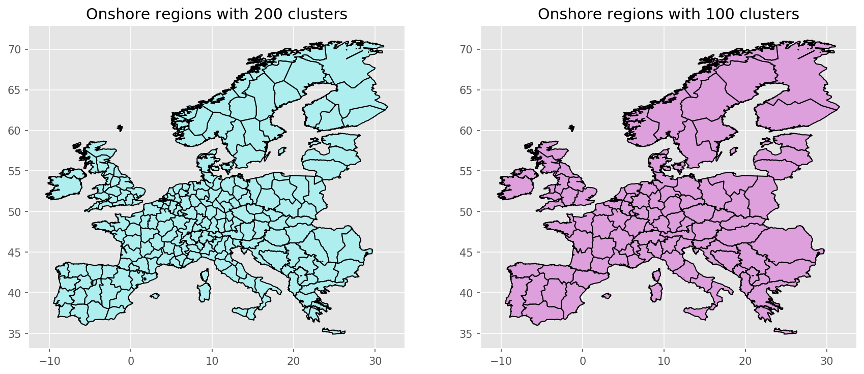

  

• resources/regions_offshore_elec_s{simpl}_{clusters}.geojson:

  

• resources/busmap_elec_s{simpl}_{clusters}.csv: Mapping of buses from networks/elec_s{simpl}.nc to networks/elec_s{simpl}_{clusters}.nc;

• resources/linemap_elec_s{simpl}_{clusters}.csv: Mapping of lines from networks/elec_s{simpl}.nc to networks/elec_s{simpl}_{clusters}.nc;

• networks/elec_s{simpl}_{clusters}.nc: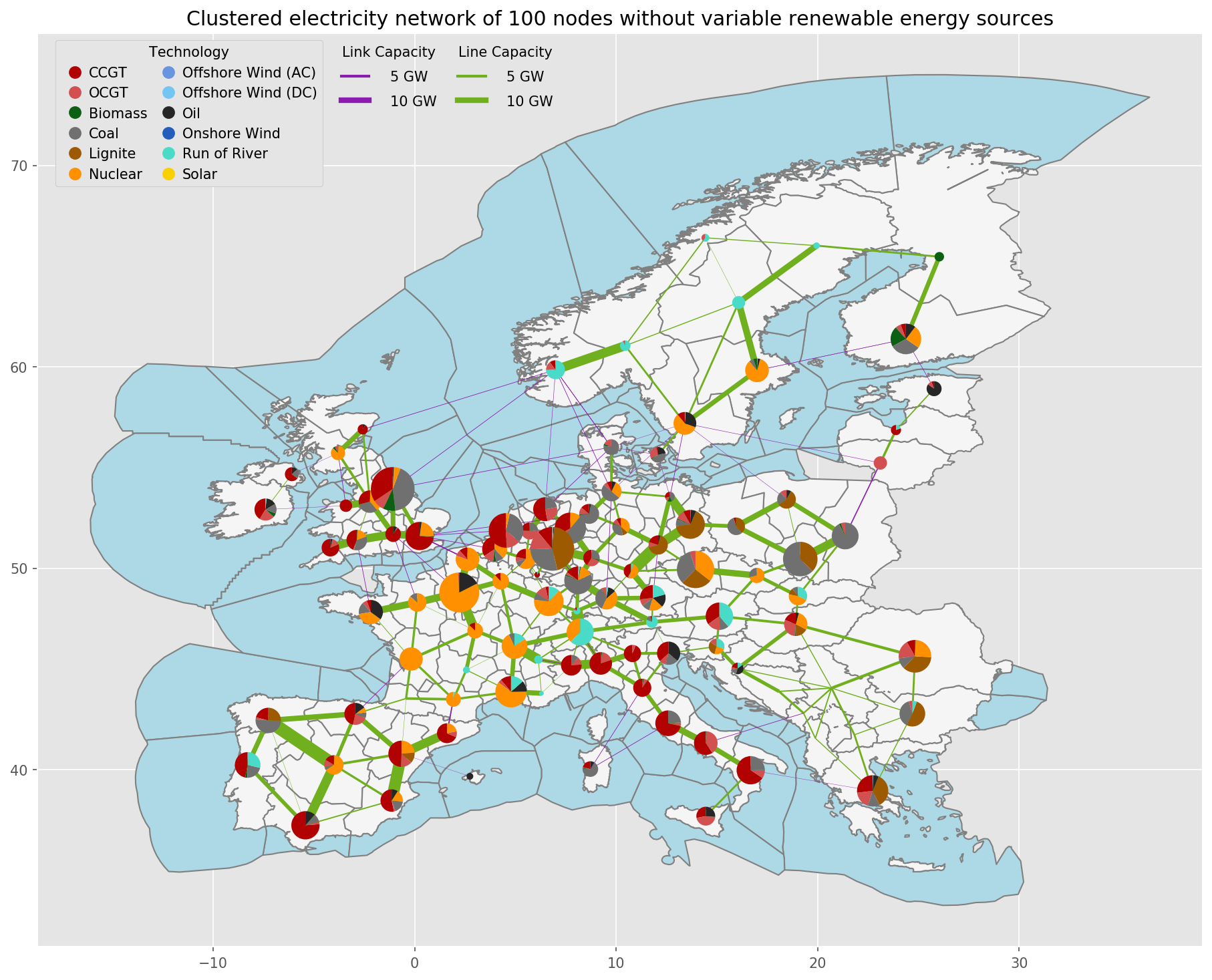

  

Description

Note

Why is clustering used both in simplify_network and cluster_network ?

Consider for example a network networks/elec_s100_50.nc in which simplify_network clusters the network to 100 buses and in a second step cluster_network` reduces it down to 50 buses.

In preliminary tests, it turns out, that the principal effect of changing spatial resolution is actually only partially due to the transmission network. It is more important to differentiate between wind generators with higher capacity factors from those with lower capacity factors, i.e. to have a higher spatial resolution in the renewable generation than in the number of buses.

The two-step clustering allows to study this effect by looking at networks like networks/elec_s100_50m.nc. Note the additional m in the {cluster} wildcard. So in the example network there are still up to 100 different wind generators.

In combination these two features allow you to study the spatial resolution of the transmission network separately from the spatial resolution of renewable generators.

Is it possible to run the model without the simplify_network rule?

No, the network clustering methods in the PyPSA module pypsa.clustering.spatial do not work reliably with multiple voltage levels and transformers.

Tip

The rule cluster_all_networks runs for all scenario s in the configuration file the rule cluster_network.

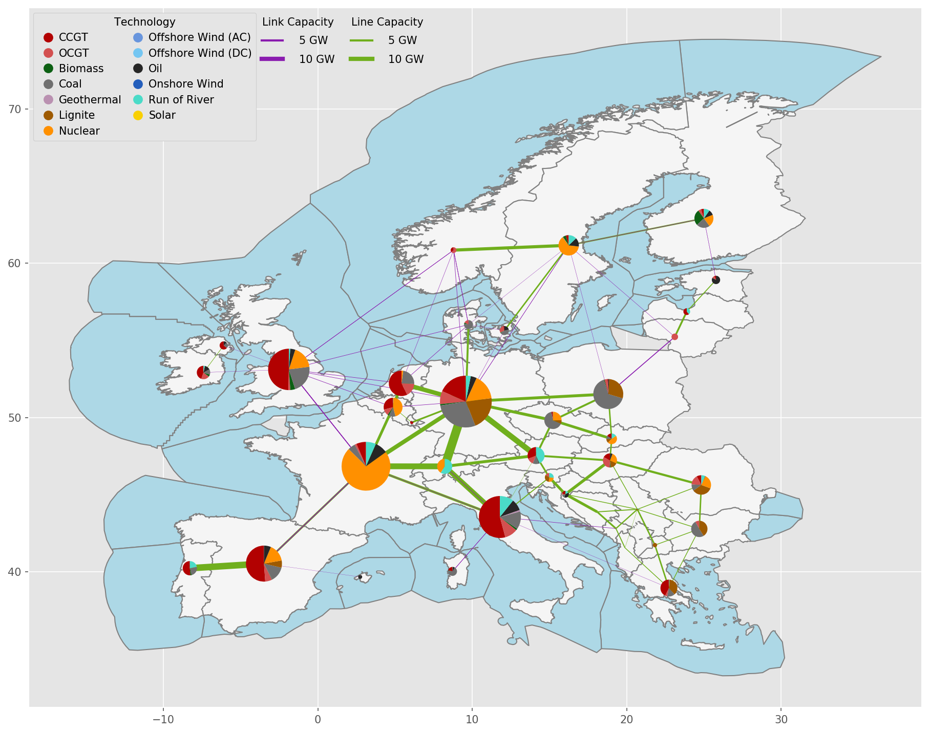
Exemplary unsolved network clustered to 512 nodes:

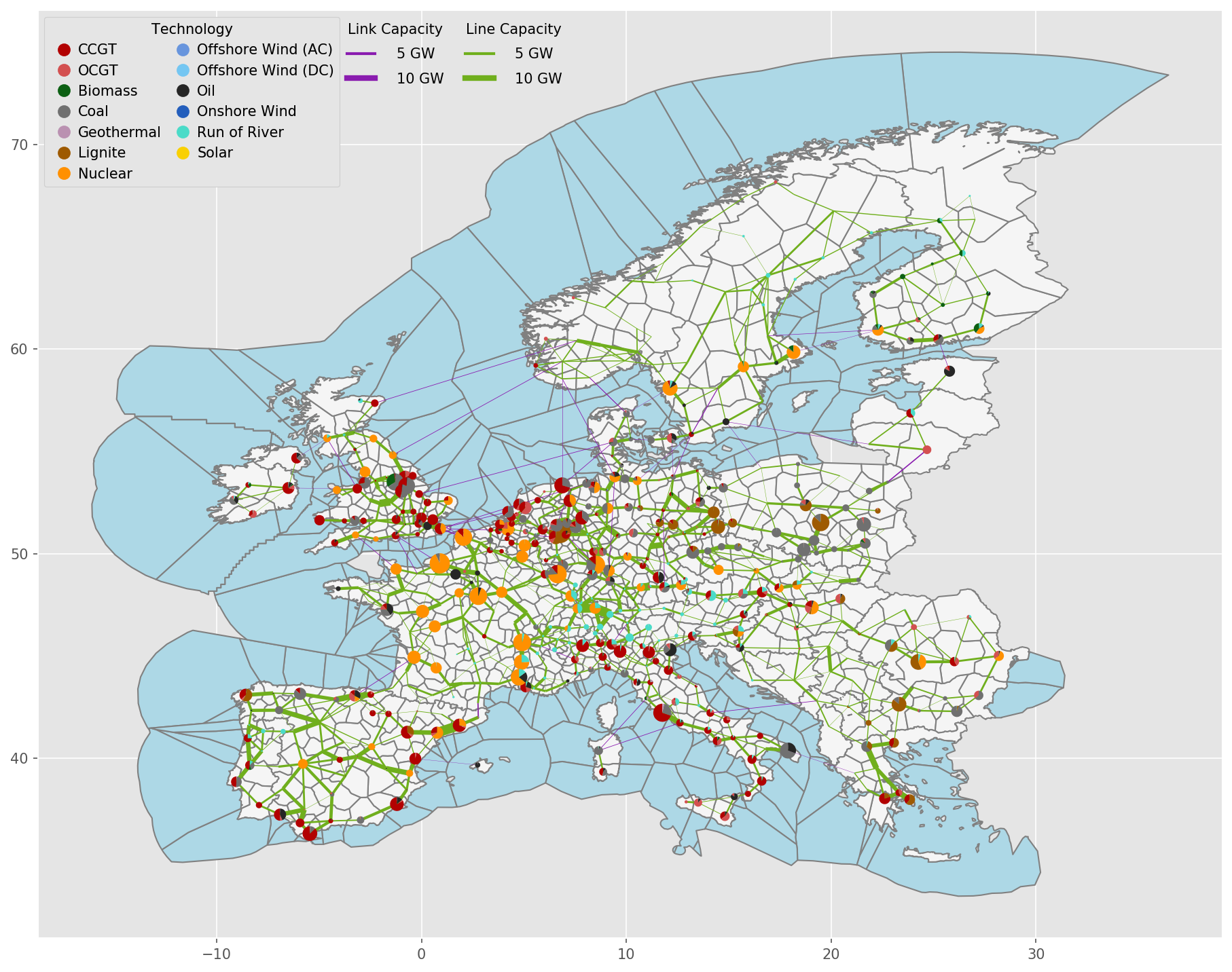
Exemplary unsolved network clustered to 256 nodes:

Exemplary unsolved network clustered to 128 nodes:

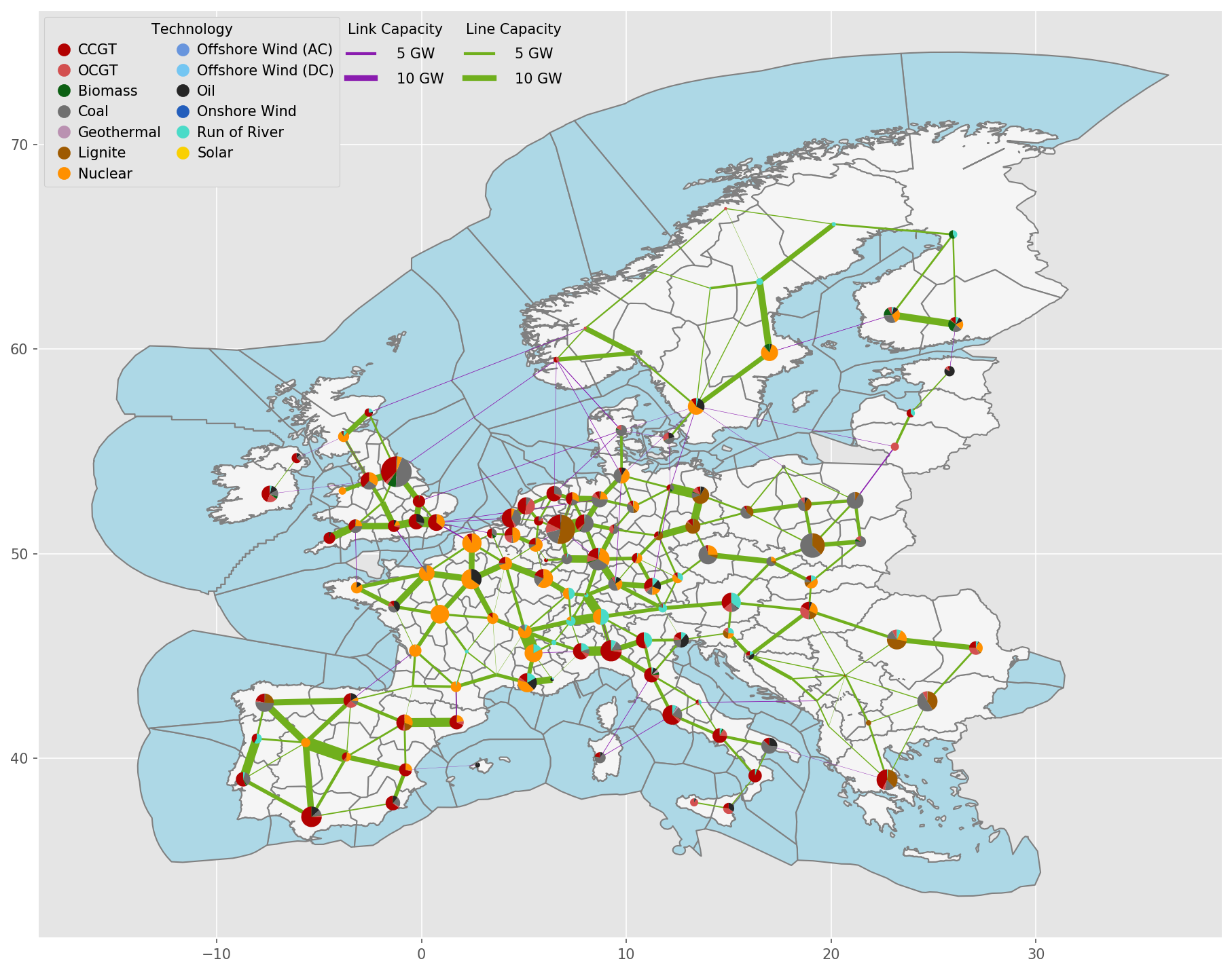
Exemplary unsolved network clustered to 37 nodes:

cluster_network.distribute_clusters(inputs, build_shape_options, country_list, distribution_cluster, n, n_clusters, focus_weights=None, solver_name=None)

Determine the number of clusters per country.

build_osm_network

build_osm_network.add_buses_to_empty_countries(country_list, fp_country_shapes, buses)

Function to add a bus for countries missing substation data.

build_osm_network.connect_stations_same_station_id(lines, buses)

Function to create fake links between substations with the same substation_id.

build_osm_network.fix_overpassing_lines(lines, buses, distance_crs, tol=1)

Function to avoid buses overpassing lines with no connection when the bus is within a given tolerance from the line.

Parameters:

• lines (GeoDataFrame) – Geodataframe of lines

• buses (GeoDataFrame) – Geodataframe of substations

• tol (float) – Tolerance in meters of the distance between the substation and the line below which the line will be split

build_osm_network.force_ac_lines(df, col='tag_frequency')

Function that forces all PyPSA lines to be AC lines.

A network can contain AC and DC power lines that are modelled as PyPSA “Line” component. When DC lines are available, their power flow can be controlled by their converter. When it is artificially converted into AC, this feature is lost. However, for debugging and preliminary analysis, it can be useful to bypass problems.

build_osm_network.get_ac_frequency(df, fr_col='tag_frequency')

# Function to define a default frequency value.

Attempts to find the most usual non-zero frequency across the dataframe; 50 Hz is assumed as a back-up value

build_osm_network.get_converters(buses, lines)

Function to create fake converter lines that connect buses of the same station_id of different polarities.

build_osm_network.get_transformers(buses, lines)

Function to create fake transformer lines that connect buses of the same station_id at different voltage.

build_osm_network.merge_stations_lines_by_station_id_and_voltage(lines, buses, geo_crs, distance_crs, tol=2000)

Function to merge close stations and adapt the line datasets to adhere to the merged dataset.

build_osm_network.merge_stations_same_station_id(buses, delta_lon=0.001, delta_lat=0.001, precision=4)

Function to merge buses with same voltage and station_id This function iterates over all substation ids and creates a bus_id for every substation and voltage level.

Therefore, a substation with multiple voltage levels is represented with different buses, one per voltage level

build_osm_network.set_lines_ids(lines, buses, distance_crs)

Function to set line buses ids to the closest bus in the list.

build_osm_network.set_lv_substations(buses)

Function to set what nodes are lv, thereby setting substation_lv The current methodology is to set lv nodes to buses where multiple voltage level are found, hence when the station_id is duplicated.

build_osm_network.set_substations_ids(buses, distance_crs, tol=2000)

Function to set substations ids to buses, accounting for location tolerance.

The algorithm is as follows:

1. initialize all substation ids to -1

2. if the current substation has been already visited [substation_id < 0], then skip the calculation

3. otherwise:

   1. identify the substations within the specified tolerance (tol)

   2. when all the substations in tolerance have substation_id < 0, then specify a new substation_id

   3. otherwise, if one of the substation in tolerance has a substation_id >= 0, then set that substation_id to all the others; in case of multiple substations with substation_ids >= 0, the first value is picked for all

clean_osm_data

config_osm_data

download_osm_data

simplify_network

make_statistics