Configuration

PyPSA-Earth is using configuration files as an interface which allows to customise a data preparation and modelling workflow. The options here described are collected in a config.yaml file located in the root directory. Users should copy the provided default configuration (config.default.yaml) and amend their own modifications and assumptions in the user-specific configuration file (config.yaml); confer installation instructions at Installation.

Top-level configuration

version: 0.8.0
tutorial: false

logging:
  level: INFO
  format: "%(levelname)s:%(name)s:%(message)s"

results_dir: results/
summary_dir: results/

foresight: overnight


countries: ["NG", "BJ"]
# Can be replaced by country ["NG", "BJ"], continent ["Africa"] or user-specific region, see more at https://pypsa-earth.readthedocs.io/en/latest/configuration.html#top-level-configuration

enable:
  retrieve_databundle: true #  Recommended 'true', for the first run. Otherwise data might be missing.
  retrieve_databundle_sector: true
  retrieve_cost_data: true # true: retrieves cost data from technology data and saves in resources/costs.csv, false: uses cost data in data/costs.csv
  download_osm_data: true # If 'true', OpenStreetMap data will be downloaded for the above given countries
  download_global_buildings: false # If 'true', GlobalMLBuildingFootprints data will be downloaded for the above given countries
  build_natura_raster: false # If 'true', then an exclusion raster will be build. Otherwise use pregenerated raster.
  build_cutout: false

	Unit	Values	Description
version	–	0.x.x	Version of PyPSA-Earth
tutorial	bool	{True, False}	Switch to retrieve the tutorial data set instead of the full data set.
logging
– level	–	Any of {‘INFO’, ‘WARNING’, ‘ERROR’}	Restrict console outputs to all infos, warning or errors only
– format	–		Custom format for log messages. See LogRecord attributes.
countries	–	Any two-letter country code on earth (60% are working, the team works on making it 100%), any continent, or any user-specific region	World countries defined by their Two-letter country codes (ISO 3166-1) which should be included in the energy system model.
enable
– retrieve_databundle	bool	{True, False}	Switch to retrieve databundle from zenodo via the rule retrieve_databundle_light or whether to keep a custom databundle located in the corresponding folder.
– retrieve_cost_data	bool	{True, False}	True: retrieves cost data from technology data and saves in resources/costs.csv, false: uses cost data in data/costs.csv
– download_osm_data	bool	{True, False}	True: OpenStreetMap data will be downloaded for the above given countries.
– build_natura_raster	bool	{True, False}	Switch to enable the creation of the raster natura.tiff via the rule build_natura_raster.
– retrieve_cutout	bool	{True, False}	Switch to retrieve cutout_databundle from gdrive via the rule retrieve_databundle_light.
– build_cutout	bool	{True, False}	Switch to enable the building of cutouts via the rule build_cutout.
custom_rules	list	Empty in case no custom rules are needed [], otherwise e.g. [“my_folder/my_rules.smk”]	Enable the addition of custom rules to the Snakefile

run

It is common to analyse energy system optimisation models for multiple scenarios for a variety of reasons, e.g. assessing their sensitivity towards changing the temporal and/or geographical resolution or investigating how investment changes as more ambitious greenhouse-gas emission reduction targets are applied.

The run section is used for running and storing scenarios with different configurations which are not covered by Wildcards. It determines the path at which resources, networks and results are stored. Therefore the user can run different configurations within the same directory. If a run with a non-empty name should use cutouts shared across runs, set shared_cutouts to true.

run:
  name: "" # use this to keep track of runs with different settings
  sector_name: "" # use this to keep track of sector scenario runs
  shared_cutouts: true # set to true to share the default cutout(s) across runs

	Unit	Values	Description
name	string		Keeps track of runs with different settings.
shared_cutouts	bool	{True, False}	True: shares the default cutout(s) across runs. Note: value false requires build_cutout to be enabled.

scenario

The scenario section is an extraordinary section of the config file that is strongly connected to the Wildcards and is designed to facilitate running multiple scenarios through a single command

snakemake -j 1 solve_all_networks

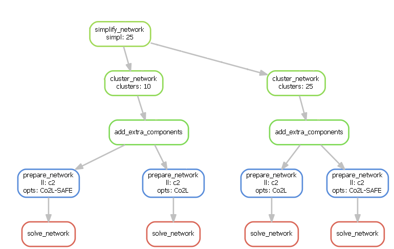
For each wildcard, a list of values is provided. The rule solve_all_networks will trigger the rules for creating results/networks/elec_s{simpl}_{clusters}_ec_l{ll}_{opts}.nc for all combinations of the provided wildcard values as defined by Python’s itertools.product(…) function that snakemake’s expand(…) function uses.

An example dependency graph (starting from the simplification rules) looks like this:

scenario:
  simpl: [""]
  ll: ["copt"]
  clusters: [10]
  opts: [Co2L-3h]

	Unit	Values	Description
simpl	–	cf. The {simpl} wildcard	List of {simpl} wildcards to run.
ll	–	cf. The {ll} wildcard	List of {ll} wildcards to run.
clusters	–	cf. The {clusters} wildcard	List of {clusters} wildcards to run.
opts	–	cf. The {opts} wildcard	List of {opts} wildcards to run.

snapshots

Specifies the temporal range for the historical weather data, which is used to build the energy system model. It uses arguments to pandas.date_range. The date range must be in the past (before 2022). A well-tested year is 2013.

snapshots:
  start: "2013-01-01"
  end: "2014-01-01"
  inclusive: "left" # end is not inclusive

	Unit	Values	Description
start	–	str or datetime-like; e.g. YYYY-MM-DD	Left bound of date range. Has to be in the past as weather and demand data for that year is required.
end	–	str or datetime-like; e.g. YYYY-MM-DD	Right bound of date range. Has to be in the past as weather and demand data for that year is required.
closed	–	One of {None, ‘left’, ‘right’}	Make the time interval closed to the left, right, or both sides None.

crs

Defines the coordinate reference systems (crs).

crs:
  geo_crs: EPSG:4326 # general geographic projection, not used for metric measures. "EPSG:4326" is the standard used by OSM and google maps
  distance_crs: EPSG:3857 # projection for distance measurements only. Possible recommended values are "EPSG:3857" (used by OSM and Google Maps)
  area_crs: ESRI:54009 # projection for area measurements only. Possible recommended values are Global Mollweide "ESRI:54009"

	Unit	Values	Description
geo_crs		General geographic projection. Not used for metric measures.	Recommended value is ‘EPSG:4326’ (used by OSM and Google Maps).
distance_crs		Projection for distance measurements only.	Recommended value is ‘EPSG:3857’ (used by OSM and Google Maps).
area_crs		Projection for area measurements only.	Recommended value is the Global Mollweide projection ‘ESRI:54009’.

natura

If enabled, build_natura_raster creates an updated raster of the wold protected areas instead of using the provided default raster in data/natura/natura.tiff. The options below select which regions to include in the raster and configure the rasterization process itself.

natura: # only relevant when using build_natura_raster: true
  natura_size: countries # countries, cutout, or global. Select which regions to include in the natura raster.
  natura_resolution: 100 # [m] Grid resolution of the natura data.
  window_size: 10000 # [bytes] Size of the shifting rasterization window. The required RAM scales with window_size^2.
  buffer_size: 10000 # [unit of area_crs, default: m] Buffer around the regions of interest to include every required value. A buffer of around 100 km will be sufficient for most cases.

	Unit	Values	Description
natura_size	string	{countries, cutout, global}	Select which regions to include in the natura raster. Either include all selected countries (counties), the entire cutout (cutout) or the entire globe (global).
natura_resolution	int		[m] Grid resolution of the natura output data.
window_size	int		[bytes] Size of the shifting rasterization window. The required RAM scales with window_size^2
buffer_size	int		[unit of area_crs, default: m] Buffer around the regions of interest to include every required value. A buffer of around 100 km will be sufficient for most cases.

augmented_line_connection

If enabled, it increases the connectivity of the network. It makes the network graph k-edge-connected, i.e., if fewer than k edges are removed, the network graph stays connected. It uses the k-edge-augmentation algorithm from the NetworkX Python package.

augmented_line_connection:
  add_to_snakefile: false # If True, includes this rule to the workflow
  connectivity_upgrade: 2 # Min. lines connection per node,
  # https://networkx.org/documentation/stable/reference/algorithms/generated/networkx.algorithms.connectivity.edge_augmentation.k_edge_augmentation.html#networkx.algorithms.connectivity.edge_augmentation.k_edge_augmentation
  new_line_type: ["HVAC"] # Expanded lines can be either ["HVAC"] or ["HVDC"] or both ["HVAC", "HVDC"]
  min_expansion: 1 # [MW] New created line expands by float/int input
  min_DC_length: 600 # [km] Minimum line length of DC line

	Unit	Values	Description
add_to_snakefile	bool	{True, False}	True: includes this rule to the workflow.
connectivity_upgrade	int	{1, 2, 3, …}	Number k such that the network graph is k-edge-connected.
new_line_type		{[“HVAC”], [“HVDC”], [“HVAC”, “HVDC”]}	Type of expanded lines.
min_expansion	int or float		[MW] New created line capacity.
min_DC_length	int or float		[km] Minimum line length of HVDC line.

cluster_options

Specifies the options to simplify and cluster the network. This is done in two stages, first using the rule simplify_network and then using the rule cluster_network. For more details on this process, see the PyPSA-Earth paper, section 3.7.

cluster_options:
  simplify_network:
    to_substations: false # network is simplified to nodes with positive or negative power injection (i.e. substations or offwind connections)
    algorithm: kmeans # choose from: [hac, kmeans]
    feature: solar+onwind-time # only for hac. choose from: [solar+onwind-time, solar+onwind-cap, solar-time, solar-cap, solar+offwind-cap] etc.
    exclude_carriers: []
    remove_stubs: true
    remove_stubs_across_borders: false
    p_threshold_drop_isolated: 20 # [MW] isolated (sub)networks or nodes are being discarded if total mean power is below the specified threshold
    p_threshold_merge_isolated: 300 # [MW] isolated (sub)networks or nodes are being merged into a single isolated bus if total mean power is below the specified threshold
    s_threshold_fetch_isolated: false # [-] a share of the national load for merging an isolated network into a backbone network
  cluster_network:
    algorithm: kmeans
    feature: solar+onwind-time
    exclude_carriers: []
  alternative_clustering: false # "False" use Voronoi shapes, "True" use GADM shapes
  distribute_cluster: ["load"] # Distributes cluster nodes per country according to ['load'],['pop'] or ['gdp']
  out_logging: true # When "True", logging is printed to console
  aggregation_strategies:
    generators: # use "min" for more conservative assumptions
      p_nom: sum
      p_nom_max: sum
      p_nom_min: sum
      p_min_pu: mean
      p_max_pu: weighted_average
      marginal_cost: mean
      committable: any
      ramp_limit_up: max
      ramp_limit_down: max
      efficiency: mean

	Unit	Values	Description
simplify_network
– to_substations	bool	{True, False}	False: network is simplified to nodes with positive or negative power injection (i.e. substations or offwind connections).
– algorithm		{hac, kmeans, modularity}	Clustering algorithm used in the simplify_network rule. Options available are Hierarchical Agglomerative Clustering (HAC), k-means, or greedy modularity.
– feature		Str in the format ‘carrier1+carrier2+…+carrierN-X’, where CarrierI can be from {‘solar’, ‘onwind’, ‘offwind’, ‘ror’} and X is one of {‘cap’, ‘time’}. Examples: solar+offwind-cap, solar-time	Only for Hierarchical Agglomerative Clustering (HAC). Feature(s) used to do the clustering.
– exclude_carriers		List of Str like [ ‘solar’, ‘onwind’] or empy list []	Carriers not considered in the simplify_network rule. Can be any set of carriers (conventional or renewable).
– remove_stubs	bool	{True, False}	True: Stub lines and links, i.e. dead-ends of the network, are sequentially removed from the network.
– remove_stubs_across_borders	bool	{True, False}	True: Stub lines and links can be removed across borders.
– p_threshold_drop_isolated	MW	positive number	Isolated buses are discarded if bus mean power is below the p_threshold_drop_isolated.
– p_threshold_merge_isolated	MW	positive number	Isolated buses are merged into a single isolated bus if bus mean power is below p_threshold_merge_isolated.
– s_threshold_fetch_isolated	[-]	positive number	Isolated networks are merged into a backbone network of a respective country if the network load comprises a share of the national load less than p_threshold_fetch_isolated.
cluster_network
– algorithm		{hac, kmeans}	Clustering algorithm used in the cluster_network rule. Options available are Hierarchical Agglomerative Clustering (HAC) or k-means.
– feature		Str in the format ‘carrier1+carrier2+…+carrierN-X’, where CarrierI can be from {‘solar’, ‘onwind’, ‘offwind’, ‘ror’} and X is one of {‘cap’, ‘time’}. Examples: solar+offwind-cap, solar-time	Only for Hierarchical Agglomerative Clustering (HAC). Feature(s) used to do the clustering.
– exclude_carriers		List of Str like [ ‘solar’, ‘onwind’] or empy list []	Carriers not considered in the cluster_network rule. Can be any set of carriers (conventional or renewable).
alternative_clustering	bool	{True, False}	False: use Voronoi shapes in the clustering. True: use GADM shapes in the clustering.
distribute_cluster		{[‘load’], [‘pop’], [‘gdp’]}	Distributes cluster nodes per country according to load ([‘load’]), population ([‘pop’]) or GDP ([‘gdp’]).
out_logging	bool	{True, False}	True: Logging is printed to the console.
aggregation_strategies
– generators
– – p_nom		{min, mean, max, sum}	Indicates how the p_nom of the aggregated generator is computed from the original p_nom values. For example, if sum, then all values within each cluster are summed to represent the new generator.
– – p_nom_max		{min, mean, max, sum}	Indicates how the p_nom_max of the aggregated generator is computed from the original p_nom_max values.
– – p_nom_min		{min, mean, max, sum}	Indicates how the p_nom_min of the aggregated generator is computed from the original p_nom_min values.
– – p_min_pu		{min, mean, max, sum}	Indicates how the p_min_pu of the aggregated generator is computed from the original p_min_pu values.
– – marginal_cost		{min, mean, max, sum}	Indicates how the marginal_cost of the aggregated generator is computed from the original marginal_cost values.
– – commitable		{any}	Indicates how the commit status of the aggregated generator is set depending on the original values of the generators. Unit Commitment is currently under development, so should be left to any.
– – ramp_limit_up		{min, mean, max, sum}	Indicates how the ramp_limit_up of the aggregated generator is computed from the original ramp_limit_up values.
– – ramp_limit_down		{min, mean, max, sum}	Indicates how the ramp_limit_down of the aggregated generator is computed from the original ramp_limit_down values.
– – efficiency		{min, mean, max, sum}	Indicates how the efficiency of the aggregated generator is computed from the original efficiency values.
focus_weights		Dict consisting of {country: share} such as {NG: 0.4}	When specified, set the share of nodes allocated to each country. The sum of focus weights must be less than or equal to 1.

build_shape_options

Specifies the options to build the shapes in which the region of interest (countries) is divided.

build_shape_options:
  gadm_layer_id: 1 # GADM level area used for the gadm_shapes. Codes are country-dependent but roughly: 0: country, 1: region/county-like, 2: municipality-like
  simplify_tolerance: 0.01 # Default value is 0.01, higher the value more is the simplification of the GADM shapes
  simplify_gadm: true # When true, shape polygons are simplified else no
  minarea: 0.01 # Minimum area of polygons to be retained in GADM shapes after simplification, in square degrees. Polygons with area smaller than this value will be removed
  update_file: false # When true, all the input files are downloaded again and replace the existing files
  out_logging: true # When true, logging is printed to console
  year: 2020 # reference year used to derive shapes, info on population and info on GDP
  nprocesses: 3 # number of processes to be used in build_shapes
  worldpop_method: "standard" # "standard" pulls from web 1kmx1km raster, "api" pulls from API 100mx100m raster,
  # false (not "false") no pop addition to shape which is useful when generating only cutout
  gdp_method: "standard" # "standard" pulls from web 1x1km raster, false (not "false") no gdp addition to shape which useful when generating only cutout
  contended_flag: "set_by_country" # "set_by_country" assigns the contended areas to the countries according to the GADM database, "drop" drops these contended areas from the model

subregion

If enabled, this option allows a region of interest (countries) to be redefined into subregions, which can be activated at various stages of the workflow. Currently, it is used in simplify_network and cluster_network rule.

subregion:
  enable:
    simplify_network: true # activate subregion in simplify_network
    cluster_network: false # activate subregion in cluster_network
  define_by_gadm: false # name of the subregion. Multiple countries can be part in the same subregion.
  path_custom_shapes: false # (optional) provide the specific absolute path of the custom file e.g. (...\data\custom_shapes.geojson)

	Unit	Values	Description
enable
– simplify_network	bool	{True, False}	Enables subregion definitions in simplify_network, allowing network simplification functions to drop or merge nodes based on subregions rather than just countries.
– cluster_network	bool	{True, False}	Enables subregion definitions in cluster_network, allowing focus_weights to set clustering focus based on subregion names.
define_by_gadm
– {subregion_name}		Str: list	Specifies the names of subregions and its GADM IDs as a list
path_custom_shapes		path	(optional) Specifies the subregion based on a custom shapes
tolerance	km	int	Buffer distance for assigning a country/subregion shape to a bus (the default tolerance is 100 km)

The names of subregions are arbitrary. Its sizes are determined by the number of GADM IDs included in the list. A single country can be divided into multiple subregions, and a single subregion can include GADM IDs from multiple countries. If the same GADM ID appears in different subregions, the first subregion listed will take precedence over that region. The remaining GADM IDs that are not listed will be merged back to form the remaining parts of their respective countries. For example, consider the Central District of Botswana, which has a GADM ID of BW.3. To separate this district from the rest of the country, you can select:

subregion:
  enable:
    simplify_network: true # activate subregion in simplify_network
    cluster_network: true # activate subregion in cluster_network
  define_by_gadm:
    Central: [BW.3]

focus_weights:
  BW: 0.7
  Central: 0.3

There are several formats for GADM IDs depending on the version, so before using this feature, please review the resources/shapes/gadm_shape.geojson file which can be created using the command:

snakemake -j 1 build_shapes

Note

The rule build_shapes currently use Version 4.1 for their GADM data. This may change in the future.

clean_osm_data_options

Specifies the options to clean the OpenStreetMap (OSM) data.

clean_osm_data_options: # osm = OpenStreetMap
  names_by_shapes: true # Set the country name based on the extended country shapes
  threshold_voltage: 51000 # [V] minimum voltage threshold to keep the asset (cable, line, generator, etc.) [V]
  tag_substation: "transmission" # Filters only substations with 'transmission' tag, ('distribution' also available)
  add_line_endings: true # When "True", then line endings are added to the dataset of the substations
  generator_name_method: OSM # Methodology to specify the name to the generator. Options: OSM (name as by OSM dataset), closest_city (name by the closest city)

build_osm_network

Specifies the options to build the OpenStreetMap (OSM) network.

build_osm_network: # Options of the build_osm_network script; osm = OpenStreetMap
  group_close_buses: true # When "True", close buses are merged and guarantee the voltage matching among line endings
  group_tolerance_buses: 5000 # [m] (default 5000) Tolerance in meters of the close buses to merge
  split_overpassing_lines: true # When True, lines overpassing buses are splitted and connected to the bueses
  overpassing_lines_tolerance: 1 # [m] (default 1) Tolerance to identify lines overpassing buses
  force_ac: false # When true, it forces all components (lines and substation) to be AC-only. To be used if DC assets create problem.

	Unit	Values	Description
group_close_buses	bool	{True, False}	True: close buses are merged and guarantee the voltage matching among line endings.
group_tolerance_buses	m		Tolerance in meters of the close buses to merge.
split_overpassing_lines	bool	{True, False}	True: lines overpassing buses are splitted and connected to the buses.
overpassing_lines_tolerance	m		Tolerance to identify lines overpassing buses.
force_ac	bool	{True, False}	True: forces all components (lines and substation) to be AC-only. To be used if DC assets create problems.

base_network

Specifies the minimum voltage magnitude in the base network and the offshore substations.

base_network:
  min_voltage_substation_offshore: 51000 # [V] minimum voltage of the offshore substations
  min_voltage_rebase_voltage: 51000 # [V] minimum voltage in base network

	Unit	Values	Description
min_voltage_substation_offshore	V		Minimum voltage magnitude in offshore substations.
min_voltage_rebase_voltage	V		Minimum voltage magnitude in base network.

load_options

Specifies the options to estimate future electricity demand (load). Different years might be considered for weather and the socioeconomic pathway (GDP and population growth), to enhance modelling capabilities.

load_options:
  ssp: "ssp2-2.6" # shared socio-economic pathway (GDP and population growth) scenario to consider
  weather_year: 2013 # Load scenarios available with different weather year (different renewable potentials)
  prediction_year: 2030 # Load scenarios available with different prediction year (GDP, population)
  scale: 1 # scales all load time-series, i.e. 2 = doubles load

	Unit	Values	Description
ssp			Scenario considered for shared socio-economic pathway (GDP and population growth).
weather_year		past year; e.g. YYYY	Year from which weather data is taken. Must be a year in the past. Well-tested years are 2011, 2013, and 2018.
prediction_year		year (can be in the future); e.g. YYYY”	Year for which the load scenario is computed (GDP and population). Well-tested years are 2030, 2040, 2050, and 2100.
scale		float	Scale for all the load time-series or specific countries if specified. For example, ‘2’ doubles the load and ‘NG: 2’ doubles the load only for Nigeria.

Warning

The snapshots date range (snapshots\start - snapshots\end) must be in the weather_year.

co2_budget

If enabled, this option allows setting different CO₂ targets for each planning horizon year. Only supports foresights with planning horizon such as myopic.

co2_budget:
  enable: false
  override_co2opt: true
  co2base_value: co2limit # choose from: [co2limit, co2base, absolute, {float}]
  year:
    2020: 1.0
    2025: 0.85
    2030: 0.70
    2035: 0.55
    2040: 0.40
    2045: 0.25
    2050: 0.1

	Unit	Values	Description
enable		{True, False}	Switch to select whether to activate this feature.
override_co2opts		{True, False}	Switch to select whether to the new co2 limits can override existing previous co2 options.
co2base_value	\(t_{CO_2-eq}/a\)	{“co2limit”, “co2base”, “absolute”, float}	The total system annual carbon dioxide equivalent emissions. The value can be provided as is, refer to existing CO₂ values, or if ‘absolute’ is selected, be defined for each planning horizon
year		Dictionary with planning horizons as keys	CO₂ budget as a fraction of co2base_value. If absolute is selected, then the total emission is set per planning horizons year

electricity

Specifies the options for the rule add_electricity. This includes options across several features, including but not limited to: voltage levels, electricity carriers available, renewable capacity estimation, CO2 emission limits, operational reserve, storage parameters. See the table below for more details.

electricity:
  base_voltage: 380.
  voltages: [132., 220., 300., 380., 500., 750.]
  co2limit: 7.75e+7 # European default, 0.05 * 3.1e9*0.5, needs to be adjusted for Africa
  co2base: 1.487e+9 # European default, adjustment to Africa necessary
  agg_p_nom_limits: # enables to set country-wise maximum and minimum generation capacities for generators (e.g. renewables, nuclear, and geothermal)
    file: data/agg_p_nom_minmax.csv # path to csv file containing country-wise generation capacity limits
    include_existing: false # false: only new built capacities are constrained; true: existing capacities are accounted in the constraints
  hvdc_as_lines: false # should HVDC lines be modeled as `Line` or as `Link` component?
  automatic_emission: false
  automatic_emission_base_year: 1990 # 1990 is taken as default. Any year from 1970 to 2018 can be selected.

  operational_reserve: # like https://genxproject.github.io/GenX/dev/core/#Reserves
    activate: false
    epsilon_load: 0.02 # share of total load
    epsilon_vres: 0.02 # share of total renewable supply
    contingency: 0 # fixed capacity in MW

  max_hours:
    battery: 6
    H2: 168

  extendable_carriers:
      # Note: For landlocked countries (e.g., Jordan, Austria, Switzerland), remove 'offwind-ac' and 'offwind-dc'
          # from the Generator list below, as these offshore wind technologies require coastline access.
    Generator: [solar, onwind, offwind-ac, offwind-dc, OCGT]
    StorageUnit: [] # battery, H2
    Store: [battery, H2]
    Link: [] # H2 pipeline

  powerplants_filter: (DateOut >= 2022 or DateOut != DateOut)
  custom_powerplants: false #  "false" use only powerplantmatching (ppm) data, "merge" combines ppm and custom powerplants, "replace" use only custom powerplants

  conventional_carriers: [nuclear, oil, OCGT, CCGT, coal, lignite, geothermal, biomass]
  renewable_carriers: [solar, onwind, offwind-ac, offwind-dc, hydro]

  estimate_renewable_capacities:
    stats: "irena" # False, = greenfield expansion, 'irena' uses IRENA stats to add expansion limits
    year: 2023 # Reference year, available years for IRENA stats are 2000 to 2023
    p_nom_min: 1 # any float, scales the minimum expansion acquired from stats, i.e. 110% of <years>'s capacities => p_nom_min: 1.1
    p_nom_max: false # sets the expansion constraint, False to deactivate this option and use estimated renewable potentials determine by the workflow, float scales the p_nom_min factor accordingly
    technology_mapping:
      # Wind is the Fueltype in ppm.data.Capacity_stats, onwind, offwind-{ac,dc} the carrier in PyPSA-Earth
      Offshore: [offwind-ac, offwind-dc]
      Onshore: [onwind]
      PV: [solar]

	Unit	Values	Description
base_voltage	kV	float	Base voltage to which all lines are simplified/aggregated. Simplification preserves transmission capacities.
voltages	kV	A subset of ‘standard’ voltages considered to map OSM-extracted voltages into ‘standard’ linetypes.
co2limit	\(t_{CO_2-eq}/a\)	float	Cap on system total annual carbon dioxide equivalent emissions.
co2base	\(t_{CO_2-eq}/a\)	float	Reference value of system total annual carbon dioxide equivalent emissions. Used only if relative emission reduction target is specified in {opts} wildcard.
automatic_emission	bool	{True, False}	True: Emissions are obtained from automatic emission extraction procedure. False: Emissions are obtained manually
automatic_emission_base_year		integer	CO2 emissions of year 1990 from EDGAR category 1A1a (Public electricity and heat production).
agg_p_nom_limits			Configure per carrier generator capacity constraints limiting minimum and maximum values of the expanded capacity p_nom_opt for individual countries. Is enabled if 'CCL' is present in {opts} wildcard.
– file	file	path	Reference to .csv file that specifies per carrier generator nominal capacity constraints for individual countries. Default is data/agg_p_nom_minmax.csv.
– include_existing	bool	{True, False}	True: Existing capacities are considered in the CCL constraints. False: Existing capacities are not considered in the CCL constraints. Default is false.
hvdc_as_lines	bool	{True, False}	True: HVDC cables are modelled as PyPSA Line components. False: HVDC cables are modeled as PyPSA Link components.
operational_reserve			The total operational reserve requirements consist of three components: epsilon_load, epsilon_vres, contingency. See GenX for more details.
– activate	bool	{True, False}	True: Operational reserve requirements are considered in the model.
– epsilon_load	float	[0, 1]	Share of total load that is required for operational reserve.
– epsilon_vres	float	[0, 1]	Share of total renewable supply that is required for operational reserve.
– contingency	MW		Operational reserve added as a contigency. For example, 5000 adds 5000 MW to the operational reserve requirements.
max_hours
– battery	hours		Amount of time it takes to fully charge batteries from empty if done at maximum power rate. See PyPSA documentation. It is used in the rule add_extra_components.
– H2	hours		Amount of time it takes to fully charge hydrogen storage from empty if done at maximum power rate. See PyPSA documentation. It is used in the rule add_extra_components.
extendable_carriers
– Generator	–	Any subset of {OCGT,CCGT}	Adds extendable OCGT and/or CCGT in nodes where gas power plants are located today without capacity limits. Note that solar, onwind, offwind-ac, offwind-dc are extendable by default according to their potentials. It is used in the add_electricity rule.
– StorageUnit	–	Any subset of {battery, H2}	Adds extendable storage units (battery and/or hydrogen) at every node/bus after clustering without capacity limits and with zero initial capacity. It is used in the add_extra_components rule.
– Store	–	Any subset of {battery,H2}	Adds extendable storage units (battery and/or hydrogen) at every node/bus after clustering without capacity limits and with zero initial capacity.
– Link	–	Any subset of {H2 pipeline}	Adds extendable links (H2 pipelines only) at every connection where there are lines or HVDC links without capacity limits and with zero initial capacity. Hydrogen pipelines require hydrogen storage to be modelled as Store.
powerplants_filter	–	use pandas.query strings here, e.g. Country not in [‘Germany’]	Filter query for the default powerplant database.
custom_powerplants	–	{false, merge, replace}	Adds custom powerplants from custom_powerplants.csv: false - use only powerplantmatching (ppm) data, merge - combines ppm and custom powerplants, replace - use only custom powerplants.
conventional_carriers	–	Any subset of {nuclear, oil, OCGT, CCGT, coal, lignite, geothermal, biomass}	List of conventional power plants to include in the model from resources/powerplants.csv.
renewable_carriers	–	Any subset of {solar, onwind, offwind-ac, offwind-dc, hydro}	List of renewable power plants to include in the model from resources/powerplants.csv.
estimate_renewable_capacities
– stats		{“irena” or False}	Defines which database to use, currently only “irena” is available. “irena” uses IRENA stats to add expansion limits. False enables greenfield expansion.
– year		Any year beetween 2000 and 2023	Reference year for renewable capacities. Available years for IRENA stats are from 2000 to 2023.
– p_nom_min		float	Scales the minimum expansion acquired from stats. For example, 110% of <years>’s capacities is obtained with p_nom_min: 1.1.
– p_nom_max		float or False	sets the expansion constraint, False to deactivate this option and use estimated renewable potentials determine by the workflow, float scales the p_nom_min factor accordingly.
– technology_mapping			Maps the technologies defined in ppm.data.Capacity_stats with the carriers in PyPSA-Earth.
– – Offshore		{‘offwind-ac’, ‘offwind-dc’}
– – Onshore		{‘onwind’}
– – PV		{‘solar’}

Warning

Carriers in conventional_carriers must not also be in extendable_carriers.

lines

Specifies electricity line parameters.

lines:
  ac_types:
    132.: "243-AL1/39-ST1A 20.0"
    220.: "Al/St 240/40 2-bundle 220.0"
    300.: "Al/St 240/40 3-bundle 300.0"
    380.: "Al/St 240/40 4-bundle 380.0"
    500.: "Al/St 240/40 4-bundle 380.0"
    750.: "Al/St 560/50 4-bundle 750.0"
  dc_types:
    500.: "HVDC XLPE 1000"
  s_max_pu: 0.7
  s_nom_max: .inf
  s_nom_max_min: -.inf
  length_factor: 1.25
  under_construction: "zero" # 'zero': set capacity to zero, 'remove': remove, 'keep': with full capacity

	Unit	Values	Description
ac_types	–	Values should specify a line type in PyPSA for AC lines. Keys should specify the corresponding voltage level (e.g. 220., 300. and 380. kV)	Specifies line types to assume for the different voltage levels of the target region. Should normally handle voltage levels 220, 300, and 380 kV.
dc_types	–	Values should specify a line type in PyPSA for DC-lines. Keys should specify the corresponding voltage level (e.g. 220., 300. and 380. kV)	Specifies DC-line types.
s_max_pu	–	Value in [0.,1.]	Correction factor for line capacities (s_nom) to approximate \(N-1\) security and reserve capacity for reactive power flows
s_nom_max	MW	float	Global upper limit for the maximum capacity of each extendable line.
s_nom_max_min	MW	float	Global lower limit for the maximum capacity of each extendable line.
length_factor	–	float	Correction factor to account for the fact that buses are not connected by lines through air-line distance.
under_construction	–	One of {‘zero’: set capacity to zero, ‘remove’: remove completely, ‘keep’: keep with full capacity}	Specifies how to handle lines which are currently under construction.

links

Specifies Link parameters. Links are a fundamental component of PyPSA .

links:
  p_max_pu: 1.0
  p_nom_max: .inf
  p_nom_max_min: -.inf
  under_construction: "zero" # 'zero': set capacity to zero, 'remove': remove, 'keep': with full capacity

	Unit	Values	Description
p_max_pu	–	Value in [0.,1.]	Correction factor for link capacities p_nom.
p_nom_max	MW	float	Global upper limit for the maximum capacity of each extendable DC link.
p_nom_max_min	MW	float	Global lower limit for the maximum capacity of each extendable DC link.
under_construction	–	One of {‘zero’, ‘remove’, ‘keep’}	Specifies how to handle lines which are currently under construction. ‘zero’: set capacity to zero; ‘remove’: remove completely, ‘keep’: keep with full capacity.

transformers

Specifies transformers parameters and types.

transformers:
  x: 0.1
  s_nom: 2000.
  type: ""

	Unit	Values	Description
x	p.u.	float	Series reactance (per unit, using s_nom as base power of the transformer. Overwritten if type is specified.
s_nom	MVA	float	Limit of apparent power which can pass through branch. Overwritten if type is specified.
type	–	A transformer type in PyPSA.	Specifies transformer types to assume for the transformers of the ENTSO-E grid extraction.

atlite

Define and specify the atlite.Cutout used for calculating renewable potentials and time-series. All options except for features are directly used as cutout parameters.

atlite:
  nprocesses: 4
  cutouts:
    cutout-2013-era5:
      module: era5
      dx: 0.3 # cutout resolution
      dy: 0.3 # cutout resolution
      # The cutout time is automatically set by the snapshot range. See `snapshot:` option above and 'build_cutout.py'.
      # time: ["2013-01-01", "2014-01-01"]  # to manually specify a different weather year (~70 years available)
      # The cutout spatial extent [x,y] is automatically set by country selection. See `countires:` option above and 'build_cutout.py'.
      # x: [-12., 35.]  # set cutout range manual, instead of automatic by boundaries of country
      # y: [33., 72]    # manual set cutout range

	Unit	Values	Description
nprocesses	–	int	Number of parallel processes in cutout preparation
cutouts
– {name}	–	Convention is to name cutouts like <region>-<year>-<source> (e.g. europe-2013-era5).	Name of the cutout netcdf file. The user may specify multiple cutouts under configuration atlite: cutouts:. Reference is used in configuration renewable: {technology}: cutout:. The cutout base may be used to automatically calculate temporal and spatial bounds of the network.
– – module	–	Subset of {‘era5’,’sarah’}	Source of the reanalysis weather dataset (e.g. ERA5 or SARAH-2)
– – x	°	Float interval within [-180, 180]	Range of longitudes to download weather data for. If not defined, it defaults to the spatial bounds of all bus shapes.
– – y	°	Float interval within [-90, 90]	Range of latitudes to download weather data for. If not defined, it defaults to the spatial bounds of all bus shapes.
– – time		Time interval within [‘1979’, ‘2018’] (with valid pandas date time strings)	Time span to download weather data for. If not defined, it defaults to the time interval spanned by the snapshots.
– – features		String or list of strings with valid cutout features (‘inlfux’, ‘wind’).	When freshly building a cutout, retrieve data only for those features. If not defined, it defaults to all available features.

renewable

Specifies the options to obtain renewable potentials in every cutout. These are divided in five different renewable technologies: onshore wind (onwind), offshore wind with AC connection (offwind-ac), offshore wind with DC connection (offwind-dc), solar (solar), and hydropower (hydro).

onwind

renewable:
  onwind:
    cutout: cutout-2013-era5
    resource:
      method: wind
      turbine: Vestas_V112_3MW
    capacity_per_sqkm: 3 # conservative, ScholzPhd Tab 4.3.1: 10MW/km^2
    # correction_factor: 0.93
    copernicus:
      # Scholz, Y. (2012). Renewable energy based electricity supply at low costs:
      #  development of the REMix model and application for Europe. ( p.42 / p.28)
      # CLC grid codes:
      # 11X/12X - Various forest types
      # 20  - Shrubs
      # 30  - Herbaceus vegetation
      # 40  - Cropland
      # 50  - Urban
      # 60  - Bare / Sparse vegetation
      # 80  - Permanent water bodies
      # 100 - Moss and lichen
      # 200 - Open sea
      grid_codes: [20, 30, 40, 60, 100, 111, 112, 113, 114, 115, 116, 121, 122, 123, 124, 125, 126]
      distance: 1000
      distance_grid_codes: [50]
    natura: true
    potential: simple # or conservative
    clip_p_max_pu: 1.e-2
    extendable: true

	Unit	Values	Description
cutout	–	Should be a file name listed in the configuration atlite: cutouts: (e.g. ‘europe-2013-era5’) or reference an existing folder in the directory cutouts. Source module must be ERA5.	Specifies the directory where the relevant weather data is stored.
resource
– method	–	Must be ‘wind’	A superordinate technology type.
– turbine	–	One of turbine types included in atlite	Specifies the turbine type and its characteristic power curve.
capacity_per_sqkm	\(MW/km^2\)	float	Allowable density of wind turbine placement.
copernicus
– grid_codes	–	Any subset of the Copernicus Land Cover code list	Specifies areas based on CLC which generally eligible for AC-connected offshore wind turbine placement.
– distance	m	int	(Optional) Distance to reserve as uneligible area around ‘distance_grid_codes’ for the renewable technology.
– distance_grid_codes	–	(Optional with ‘distance’) Any subset of the Copernicus Land Cover code list	Specifies from which a distance of ‘distance’ metres is unavailable as a buffer area.
natura	bool	{true, false}	Switch to exclude Natura 2000 natural protection areas. Area is excluded if true.
potential	–	One of {‘simple’, ‘conservative’}	Method to compute the maximal installable potential for a node; confer Rule build_renewable_profiles
clip_p_max_pu	p.u.	float	To avoid too small values in the renewables` per-unit availability time series values below this threshold are set to zero.
extendable	bool	{True, False}	True: In nodes where there is no onwind generation, adds a zero-capacity onwind generator so that onwind is considered in the capacity expansion. It is done in the add_electricity rule.

offwind-ac

  offwind-ac:
    cutout: cutout-2013-era5
    resource:
      method: wind
      turbine: NREL_ReferenceTurbine_5MW_offshore
    capacity_per_sqkm: 2
    # correction_factor: 0.8855
    # proxy for wake losses
    # from 10.1016/j.energy.2018.08.153
    # until done more rigorously in #153
    copernicus:
      grid_codes: [80, 200]
    natura: true
    max_depth: 50
    max_shore_distance: 30000
    potential: simple # or conservative
    clip_p_max_pu: 1.e-2
    extendable: true

	Unit	Values	Description
cutout	–	Should be a file name listed in the configuration atlite: cutouts: (e.g. ‘europe-2013-era5’) or reference an existing folder in the directory cutouts. Source module must be ERA5.	Specifies the directory where the relevant weather data is stored.
resource
– method	–	Must be ‘wind’	A superordinate technology type.
– turbine	–	One of turbine types included in atlite	Specifies the turbine type and its characteristic power curve.
capacity_per_sqkm	\(MW/km^2\)	float	Allowable density of wind turbine placement.
correction_factor		[0., 1.]	Wind correction factor to account for wake losses. It gets multiplied by the theoretical maximum in the cutout to account for wake losses.
copernicus
– grid_codes	–	Any subset of the Copernicus Land Cover code list	Specifies areas based on CLC which generally eligible for AC-connected offshore wind turbine placement.
natura	bool	{true, false}	Switch to exclude Natura 2000 natural protection areas. Area is excluded if true.
max_depth	m	float	Maximum sea water depth at which wind turbines can be build. Maritime areas with deeper waters are excluded in the process of calculating the AC-connected offshore wind potential.
max_shore_distance	m	float	Maximum distance to the shore beyond which wind turbines with AC connections cannot be build. Such areas far away from shore are excluded in the process of calculating the AC-connected offshore wind potential.
potential	–	One of {‘simple’, ‘conservative’}	Method to compute the maximal installable potential for a node; confer Rule build_renewable_profiles
clip_p_max_pu	p.u.	float	To avoid too small values in the renewables` per-unit availability time series values below this threshold are set to zero.
extendable	bool	{True, False}	True: In nodes where there is no offwind-ac generation, adds a zero-capacity offwind-ac generator so that offwind-ac is considered for capacity expansion. It is done in the add_electricity rule.

offwind-dc

  offwind-dc:
    cutout: cutout-2013-era5
    resource:
      method: wind
      turbine: NREL_ReferenceTurbine_5MW_offshore
    # ScholzPhd Tab 4.3.1: 10MW/km^2
    capacity_per_sqkm: 3
    # correction_factor: 0.8855
    # proxy for wake losses
    # from 10.1016/j.energy.2018.08.153
    # until done more rigorously in #153
    copernicus:
      grid_codes: [80, 200]
    natura: true
    max_depth: 50
    min_shore_distance: 30000
    potential: simple # or conservative
    clip_p_max_pu: 1.e-2
    extendable: true

	Unit	Values	Description
cutout	–	Should be a file name listed in the configuration atlite: cutouts: (e.g. ‘europe-2013-era5’) or reference an existing folder in the directory cutouts. Source module must be ERA5.	Specifies the directory where the relevant weather data is stored.
resource
– method	–	Must be ‘wind’	A superordinate technology type.
– turbine	–	One of turbine types included in atlite	Specifies the turbine type and its characteristic power curve.
capacity_per_sqkm	\(MW/km^2\)	float	Allowable density of wind turbine placement.
correction_factor		[0., 1.]	Wind correction factor to account for wake losses. It gets multiplied by the theoretical maximum in the cutout to account for wake losses.
copernicus
– grid_codes	–	Any subset of the Copernicus Land Cover code list	Specifies areas based on CLC which generally eligible for AC-connected offshore wind turbine placement.
natura	bool	{true, false}	Switch to exclude Natura 2000 natural protection areas. Area is excluded if true.
max_depth	m	float	Maximum sea water depth at which wind turbines can be build. Maritime areas with deeper waters are excluded in the process of calculating the AC-connected offshore wind potential.
min_shore_distance	m	float	Minimum distance to the shore below which wind turbines cannot be build. Such areas close to the shore are excluded in the process of calculating the AC-connected offshore wind potential.
potential	–	One of {‘simple’, ‘conservative’}	Method to compute the maximal installable potential for a node; confer Rule build_renewable_profiles
clip_p_max_pu	p.u.	float	To avoid too small values in the renewables` per-unit availability time series values below this threshold are set to zero.
extendable	bool	{True, False}	True: In nodes where there is no offwind-dc generation, adds a zero-capacity offwind-dc generator so that offwind-dc is considered for capacity expansion. It is done in the add_electricity rule.

solar

  solar:
    cutout: cutout-2013-era5
    resource:
      method: pv
      panel: CSi
      orientation: latitude_optimal # will lead into optimal design
      # slope: 0.  # slope: 0 represent a flat panel
      # azimuth: 180.  # azimuth: 180 south orientation
    capacity_per_sqkm: 4.6 # From 1.7 to 4.6 addresses issue #361
    # Determined by comparing uncorrected area-weighted full-load hours to those
    # published in Supplementary Data to
    # Pietzcker, Robert Carl, et al. "Using the sun to decarbonize the power
    # sector: The economic potential of photovoltaics and concentrating solar
    # power." Applied Energy 135 (2014): 704-720.
    correction_factor: 0.854337
    copernicus:
      grid_codes: [20, 30, 40, 50, 60, 90, 100]
    natura: true
    potential: simple # or conservative
    clip_p_max_pu: 1.e-2
    extendable: true

	Unit	Values	Description
cutout	–	Should be a file name listed in the configuration atlite: cutouts: (e.g. ‘europe-2013-era5’) or reference an existing folder in the directory cutouts. Source module can be ERA5 or SARAH-2.	Specifies the directory where the relevant weather data is stored that is specified at atlite/cutouts configuration. Both sarah and era5 work.
resource
– method	–	Must be ‘pv’	A superordinate technology type.
– panel	–	One of {‘Csi’, ‘CdTe’, ‘KANENA’} as defined in atlite	Specifies the solar panel technology and its characteristic attributes.
– orientation		use either {latitude_optimal} or options such {slope: 0, azimuth: 180}
– – latitude_optimal	–	Atlite function which returns for every raster the optimal slope and azimuth
– – slope	°	Realistically any angle in [0., 90.]	Specifies the tilt angle (or slope) of the solar panel. A slope of zero corresponds to the face of the panel aiming directly overhead. A positive tilt angle steers the panel towards the equator.
– – azimuth	°	Any angle in [0., 360.]	Specifies the azimuth orientation of the solar panel. South corresponds to 180.°.
capacity_per_sqkm	\(MW/km^2\)	float	Allowable density of solar panel placement. Value relates to socio-technical acceptable density.
correction_factor	–	float	A correction factor for the capacity factor (availability) time series.
copernicus
– grid_codes	–	Any subset of the Copernicus Land Cover code list	Specifies areas based on CLC which generally eligible for AC-connected offshore wind turbine placement.
natura	bool	{true, false}	Switch to exclude Natura 2000 natural protection areas. Area is excluded if true.
potential	–	One of {‘simple’, ‘conservative’}	Method to compute the maximal installable potential for a node; confer Rule build_renewable_profiles
clip_p_max_pu	p.u.	float	To avoid too small values in the renewables` per-unit availability time series values below this threshold are set to zero.
extendable	bool	{True, False}	True: In nodes where there is no solar generation, adds a zero-capacity solar generator so that solar is considered for capacity expansion. It is done in the add_electricity rule.

hydro

  hydro:
    cutout: cutout-2013-era5
    hydrobasins_level: 6
    resource:
      method: hydro
      hydrobasins: data/hydrobasins/hybas_world.shp
      flowspeed: 1.0 # m/s
      # weight_with_height: false
      # show_progress: true
    carriers: [ror, PHS, hydro]
    PHS_max_hours: 6
    hydro_max_hours: "energy_capacity_totals_by_country" # not active
    hydro_max_hours_default: 6.0 # (optional, default 6) Default value of max_hours for hydro when NaN values are found
    clip_min_inflow: 1.0
    extendable: true
    normalization:
      method: eia # 'hydro_capacities' to rescale country hydro production by using hydro_capacities, 'eia' to rescale by eia data, false for no rescaling
      year: 2013 # (optional) year of statistics used to rescale the runoff time series. When not provided, the cutout weather year is used
    multiplier: 1.1 # multiplier applied after the normalization of the hydro production; default 1.0

	Unit	Values	Description
cutout	–	Must be ‘europe-2013-era5’	Specifies the directory where the relevant weather data is stored.
resource
– method			Specifies the Atlite method to calculate renewable potential.
– hydrobasin			Specifies the file location for hydrobasins. They are used to make the runoff calibration, defining a polygon to compute the available water surface using a surface integral.
– flowspeed
carriers	–	Any subset of {‘ror’, ‘PHS’, ‘hydro’}	Specifies the types of hydro power plants to build per-unit availability time series for. ‘ror’ stands for run-of-river plants, ‘PHS’ represents pumped-hydro storage, and ‘hydro’ stands for hydroelectric dams.
PHS_max_hours	h	float	Maximum state of charge capacity of the pumped-hydro storage (PHS) in terms of hours at full output capacity p_nom. Cf. PyPSA documentation.
hydro_max_hours	h	Any of {float, ‘energy_capacity_totals_by_country’, ‘estimate_by_large_installations’}	Maximum state of charge capacity of the pumped-hydro storage (PHS) in terms of hours at full output capacity p_nom or heuristically determined. Cf. PyPSA documentation.
hydro_max_hours_default	h	float	(optional, default 6) Default value of max_hours for hydro plants with missing values
clip_min_inflow	MW	float	To avoid too small values in the inflow time series, values below this threshold are set to zero.
extendable	bool	{True, False}	True: In nodes where there is no hydro generation, adds a zero-capacity hydro generator so that hydro is considered for capacity expansion. It is done in the add_electricity rule.
normalization	–	dict	When specified, it describes how to normalize hydro time series to adhere to national statistics
–method	–	str	Data source used to rescale the hydro runoff; option ‘hydro_capacities’ to use the provided ‘data/hydro_capacities.csv’ or ‘eia’ for using the eia file
–year	–	year	(optional) Specify the desired year to be used for normalization, the default value corresponds to the cutout weather year
multiplier	–	float	Multiplier factor of the rescaling process (default 1.0)

csp

  csp:
    cutout: cutout-2013-era5
    resource:
      method: csp
      installation: SAM_solar_tower
    capacity_per_sqkm: 2.392 # From 1.7 to 4.6 addresses issue #361
    # Determined by comparing uncorrected area-weighted full-load hours to those
    # published in Supplementary Data to
    # Pietzcker, Robert Carl, et al. "Using the sun to decarbonize the power
    # sector: The economic potential of photovoltaics and concentrating solar
    # power." Applied Energy 135 (2014): 704-720.
    copernicus:
      grid_codes: [20, 30, 40, 60, 90]
      distancing_codes: [50]
      distance_to_codes: 3000
    natura: true
    potential: simple # or conservative
    clip_p_max_pu: 1.e-2
    extendable: true
    csp_model: advanced # simple or advanced

	Unit	Values	Description
cutout	–	Should be a file name listed in the configuration atlite: cutouts: (e.g. ‘europe-2013-era5’) or reference an existing folder in the directory cutouts. Source module can be ERA5 or SARAH-2.	Specifies the directory where the relevant weather data is stored that is specified at atlite/cutouts configuration. Both sarah and era5 work.
resource
– method	–	Must be ‘csp’
– installation	–	Should be ‘SAM_solar_tower’ as defined in atlite	Specifies the csp technology and its characteristic attributes.
capacity_per_sqkm	\(MW/km^2\)	float	Allowable density of csp tower placement. Value relates to socio-technical acceptable density.
copernicus
– grid_codes	–	Any subset of the Copernicus Land Cover code list	Specifies areas based on CLC which generally eligible for csp tower placement.
– distance	m	int	(Optional) Distance to reserve as uneligible area around ‘distance_grid_codes’ for the renewable technology.
– distance_grid_codes	–	(Optional with ‘distance’) Any subset of the Copernicus Land Cover code list	Specifies from which a distance of ‘distance’ metres is unavailable as a buffer area.
natura	bool	{true, false}	Switch to exclude Natura 2000 natural protection areas. Area is excluded if true.
potential	–	One of {‘simple’, ‘conservative’}	Method to compute the maximal installable potential for a node; confer Rule build_renewable_profiles
clip_p_max_pu	p.u.	float	To avoid too small values in the renewables` per-unit availability time series values below this threshold are set to zero.
extendable	bool	{True, False}	True: In nodes where there is no csp generation, adds a zero-capacity csp generator so that csp is considered for capacity expansion. It is done in the add_electricity rule.
csp_model	–	One of {‘advanced’ or ‘simple’}	Specifies the CSP model to be used. The advanced model attach stores and links to the csp buses while the simple has no stores and links.

costs

Specifies the cost assumptions of the technologies considered. Cost information is obtained from the config file and the file data/costs.csv, which can also be modified manually.

costs:
  year: 2030 # cost file selection, i.e. costs_2030.csv in this case; reference year for costs is always 2020
  technology_data_version: v0.13.2
  discountrate: [0.071] #, 0.086, 0.111]
  country_specific_data: "" # (optional) Reference to the desired technology-data directory for techno-economic input data; Only "" and "US" supported, for other values check the technology-data output directory
  # Only needed if "US" is selected as `country_specific_data`, otherwise ignore
  cost_scenario: "moderate" # only used if `country_specific_data: "US"`; can be "moderate", "advanced" or "conservative"
  financial_case: "market" # only used if `country_specific_data: "US"`; can be "market" or "r&d"
  # Management of output currencies and exchange rates
  output_currency: "EUR" # full list of supported currencies at https://github.com/alexprengere/currencyconverter/blob/master/currency_converter/eurofxref.csv
  default_exchange_rate: 0.7532 # previously USD2013_to_EUR2013; should be sufficient as current data from 'technology-data` are either in EUR or USD; [EUR/USD] ECB: https://www.ecb.europa.eu/stats/exchange/eurofxref/html/eurofxref-graph-usd.en.html
  future_exchange_rate_strategy: "reference" # reference uses the exchange rate from `reference_year` for all conversions, ensuring all costs are expressed in the same currency and year; "latest" uses the yearly average of the latest available exchange rates for the selected `output_currency`; "custom" allows to specify a `custom_future_exchange_rate` below
  custom_future_exchange_rate: None # if `future_exchange_rate_strategy: "custom"`, please insert here the desired output_currency-to-EUR exchange rate
  rooftop_share: 0.14 # based on the potentials, assuming (0.1 kW/m2 and 10 m2/person)
  fill_values:
    FOM: 0
    VOM: 0
    efficiency: 1
    fuel: 0
    investment: 0
    lifetime: 25
    CO2 intensity: 0
    discount rate: 0.07
  marginal_cost: # EUR/MWh
    solar: 0.01
    onwind: 0.015
    offwind: 0.015
    hydro: 0.
    H2: 0.
    electrolysis: 0.
    fuel cell: 0.
    battery: 0.
    battery inverter: 0.
  emission_prices: # in currency per tonne emission, only used with the option Ep
    co2: 0.
  # investment: # EUR/MW
  #   CCGT: 830000
  # FOM: # %/year
  #   CCGT: 3.35
  # VOM: # EUR/MWh
  #   CCGT: 4.2
  # fuel: # EUR/MWh
  #   gas: 10.1
  # lifetime: # years
  #   CCGT: 25.0
  # efficiency: # per unit
  #   CCGT: 0.58

Note

To change cost assumptions in more detail (i.e. other than marginal_cost), consider modifying cost assumptions directly in data/costs.csv as this is not yet supported through the config file. You can also build multiple different cost databases. Make a renamed copy of data/costs.csv (e.g. data/costs-optimistic.csv) and set the variable COSTS=data/costs-optimistic.csv in the Snakefile.

Note

The marginal costs or in this context variable costs of operating the assets is important for realistic operational model outputs. It can define the curtailment order of renewable generators, the dispatch order of generators, and the dispatch of storage units. If not approapriate set, the model might output unrealistic results. Learn more about this in Parzen et al. 2023 and in Kittel et al. 2022.

monte_carlo

Specifies the options for Monte Carlo sampling.

monte_carlo:
  # Description: Specify Monte Carlo sampling options for uncertainty analysis.
  # Define the option list for Monte Carlo sampling.
  # Make sure add_to_snakefile is set to true to enable Monte-Carlo
  options:
    add_to_snakefile: false # When set to true, enables Monte Carlo sampling
    samples: 9 # number of optimizations. Note that number of samples when using scipy has to be the square of a prime number
    sampling_strategy: "chaospy" # "pydoe2", "chaospy", "scipy", packages that are supported
    seed: 42 # set seedling for reproducibilty
  # Uncertanties on any PyPSA object are specified by declaring the specific PyPSA object under the key 'uncertainties'.
  # For each PyPSA object, the 'type' and 'args' keys represent the type of distribution and its argument, respectively.
  # Supported distributions types are uniform, normal, lognormal, triangle, beta and gamma.
  # The arguments of the distribution are passed using the key 'args'  as follows, tailored by distribution type
  # normal: [mean, std], lognormal: [mean, std], uniform: [lower_bound, upper_bound],
  # triangle: [mid_point (between 0 - 1)], beta: [alpha, beta], gamma: [shape, scale]
  # More info on the distributions are documented in the Chaospy reference guide...
  # https://chaospy.readthedocs.io/en/master/reference/distribution/index.html
  # An abstract example is as follows:
  # {pypsa network object, e.g. "loads_t.p_set"}:
  # type: {any supported distribution among the previous: "uniform", "normal", ...}
  # args: {arguments passed as a list depending on the distribution, see the above and more at https://pypsa.readthedocs.io/}
  uncertainties:
    loads_t.p_set:
      type: uniform
      args: [0.5, 1]
    generators_t.p_max_pu.loc[:, n.generators.carrier == "onwind"]:
      type: lognormal
      args: [1.5]
    generators_t.p_max_pu.loc[:, n.generators.carrier == "solar"]:
      type: beta
      args: [0.5, 2]

	Unit	Values	Description
options
add_to_snakemake		true or false	Set to true to enable Monte-Carlo
samples		int	Defines the number of total sample networks that will be optimized. If the chosen sampling strategy is scipy, then a square of a prime number needs to be chosen. E.g. 49 which is (7^2)
sampling_strategy		Any subset of {pydoe2, chaospy, scipy}	Current supported packages to create an experimental design
seed		int	Allows experimentation to be reproduced easily
uncertainties
<any pypsa.object syntax>	MW/MWh		Key is a dynamic PyPSA object that allows to access any pypsa object such as loads_t.p_set or the max. wind generation per hour generators_t.p_max_pu.loc[:, n.generators.carrier == “wind”]. Values or bounds are multiplication for each object.
type		str	Defines the distribution for the chosen pypsa.object parameter. Distribution can be either uniform, normal, lognormal, triangle, beta or gamma
args		list	Defines parameters for the chosen distribution. [mean, std] for normal and lognormal, [lower_bound, upper_bound] for uniform, [mid_point (between 0 - 1)] for triangle, [alpha, beta] for beta, [shape, scale] for gamma

sector

Specifies the options for the sector coupling, i.e. the integration of the electricity system with other sectors such as heating and transport.

policy_config:
  hydrogen:
    temporal_matching: "no_temporal_matching" #either "hour", "month", "year", "no_temporal_matching"
    spatial_matching: false
    temporal_matching_carriers: [csp, solar, onwind, offwind-ac, offwind-dc, ror, hydro]
    matching_technologies: ["H2 Electrolysis", "Alkaline electrolyzer large", "Alkaline electrolyzer medium", "Alkaline electrolyzer small", "PEM electrolyzer", "SOEC"]
    additionality: false # RE electricity is equal to the amount required for additional hydrogen export compared to the 0 export case ("reference_case")
    allowed_excess: 1.0
    is_reference: false # Whether or not this network is a reference case network, relevant only if additionality is _true_
    remove_h2_load: false #Whether or not to remove the h2 load from the network, relevant only if is_reference is _true_
    path_to_ref: "" # Path to the reference case network for additionality calculation, relevant only if additionality is _true_ and is_reference is _false_
    re_country_load: false # Set to "True" to force the RE electricity to be equal to the electricity required for hydrogen export and the country electricity load. "False" excludes the country electricity load from the constraint.


demand_data:
  update_data: true # if true, the workflow downloads the energy balances data saved in data/demand/unsd/data again. Turn on for the first run.
  base_year: 2019

  other_industries: false # Whether or not to include industries that are not specified. some countries have has exaggerated numbers, check carefully.
  aluminium_year: 2019 # Year of the aluminium demand data specified in `data/AL_production.csv`


fossil_reserves:
  oil: 100 #TWh Maybe redundant

export:
  endogenous: false # If true, the export demand is endogenously determined by the model
  endogenous_price: 400 # EUR/MWh # Market price, for wich the hydrogen for endogenous exports is sold. Only considered, if ["export"]["endogenous"] is set to true.
  store: true # [True, False] # specifies whether an export store to balance demand is implemented
  store_capital_costs: "no_costs" # ["standard_costs", "no_costs"] # specifies the costs of the export store. "standard_costs" takes CAPEX of "hydrogen storage tank type 1 including compressor"
  h2export: [10] # Yearly export demand in TWh. Only considered, if ["export"]["endogenous"] is set to false
  export_profile: "ship" # use "ship" or "constant". Only considered, if ["export"]["endogenous"] is set to false
  ship:
    ship_capacity: 0.4 # TWh # 0.05 TWh for new ones, 0.003 TWh for Susio Frontier, 0.4 TWh according to Hampp2021: "Corresponds to 11360 t H2 (l) with LHV of 33.3333 Mwh/t_H2. Cihlar et al 2020 based on IEA 2019, Table 3-B"
    travel_time: 288 # hours # From Agadir to Rotterdam and back (12*24)
    fill_time: 24 # hours, for 48h see Hampp2021
    unload_time: 24 # hours for 48h see Hampp2021

custom_data:
  renewables: [] # ['csp', 'rooftop-solar', 'solar']
  elec_demand: false
  heat_demand: false
  industry_demand: false
  industry_database: false
  transport_demand: false
  water_costs: false
  h2_underground: false
  add_existing: false
  custom_sectors: false
  gas_network: false # If "True" then a custom .csv file must be placed in "resources/custom_data/pipelines.csv" , If "False" the user can choose btw "greenfield" or Model built-in datasets. Please refer to ["sector"] below.
  export_ports: false # If "True" then a custom .csv file must be placed in "data/custom/export_ports.csv"
  airports: false # If "True" then a custom .csv file must be placed in "data/custom/airports.csv". Data format for aiports must be in the format of the airports.csv file in the data folder.

industry:
  reference_year: 2015

solar_thermal:
  clearsky_model: simple
  orientation:
    slope: 45.
    azimuth: 180.

existing_capacities:
  grouping_years_power: [1960, 1965, 1970, 1975, 1980, 1985, 1990, 1995, 2000, 2005, 2010, 2015, 2020, 2025, 2030]
  grouping_years_heat: [1980, 1985, 1990, 1995, 2000, 2005, 2010, 2015, 2019] # these should not extend 2020
  threshold_capacity: 10
  default_heating_lifetime: 20
  conventional_carriers:
  - lignite
  - coal
  - oil
  - uranium

sector:
  enable:
    heat: true
    biomass: true
    industry: true
    shipping: true
    aviation: true
    land_transport: true
    rail_transport: true
    agriculture: true
    residential: true
    services: true

  gas:
    spatial_gas: true # ALWAYS TRUE
    network: false # ALWAYS FALSE for now (NOT USED)
    network_data: GGIT # Global dataset -> 'GGIT' , European dataset -> 'IGGIELGN'
    network_data_GGIT_status: ["Construction", "Operating", "Idle", "Shelved", "Mothballed", "Proposed"]
  hydrogen:
    network: true
    H2_retrofit_capacity_per_CH4: 0.6
    network_limit: 2000 #GWkm
    network_routes: gas # "gas or "greenfield". If "gas"  ->  the network data are fetched from ["sector"]["gas"]["network_data"]. If "greenfield"  -> the network follows the topology of electrical transmission lines
    gas_network_repurposing: true # If true -> ["sector"]["gas"]["network"] is automatically false
    underground_storage: false
    hydrogen_colors: false
    set_color_shares: false
    blue_share: 0.40
    pink_share: 0.05
    production_technologies: ["H2 Electrolysis", "SMR", "SMR CC"] # ["Alkaline electrolyzer large", "Alkaline electrolyzer medium", "Alkaline electrolyzer small", "PEM electrolyzer", "SOEC", "Solid biomass steam reforming", "Biomass gasification", "Biomass gasification CC", "Natural gas steam reforming", "Natural gas steam reforming CC", "Coal gasification", "Coal gasification CC", "Heavy oil partial oxidation"] a list of H2 production technologies that can be added

  coal:
    spatial_coal: true
    shift_to_elec: true # If true, residential and services demand of coal is shifted to electricity. If false, the final energy demand of coal is disregarded
  lignite:
    spatial_lignite: false

  international_bunkers: false #Whether or not to count the emissions of international aviation and navigation

  oil:
    spatial_oil: true

  district_heating:
    potential: 0.3 #maximum fraction of urban demand which can be supplied by district heating
    #increase of today's district heating demand to potential maximum district heating share
    #progress = 0 means today's district heating share, progress=-1 means maximum fraction of urban demand is supplied by district heating
    progress: 1
    # 2020: 0.0
    # 2030: 0.3
    # 2040: 0.6
    # 2050: 1.0
    district_heating_loss: 0.15
  reduce_space_heat_exogenously: false # reduces space heat demand by a given factor (applied before losses in DH)
  # this can represent e.g. building renovation, building demolition, or if
  # the factor is negative: increasing floor area, increased thermal comfort, population growth
  # NB The value of space heat reduction are Europe-specific
  # if they usage is enabled (reduce_space_heat_exogenously) a regional adjustment is needed
  reduce_space_heat_exogenously_factor: 0.29 # per unit reduction in space heat demand
  # the default factors are determined by the LTS scenario from http://tool.european-calculator.eu/app/buildings/building-types-area/?levers=1ddd4444421213bdbbbddd44444ffffff11f411111221111211l212221
  # 2020: 0.10  # this results in a space heat demand reduction of 10%
  # 2025: 0.09  # first heat demand increases compared to 2020 because of larger floor area per capita
  # 2030: 0.09
  # 2035: 0.11
  # 2040: 0.16
  # 2045: 0.21
  # 2050: 0.29

  tes: true
  tes_tau: # 180 day time constant for centralised, 3 day for decentralised
    decentral: 3
    central: 180
  boilers: true
  oil_boilers: false
  chp: true
  micro_chp: false
  solar_thermal: true
  heat_pump_sink_T: 55 #Celsius, based on DTU / large area radiators; used un build_cop_profiles.py
  time_dep_hp_cop: true #time dependent heat pump coefficient of performance
  solar_cf_correction: 0.788457 # = >>>1/1.2683
  bev_plug_to_wheel_efficiency: 0.2 #kWh/km from EPA https://www.fueleconomy.gov/feg/ for Tesla Model S
  bev_charge_efficiency: 0.9 #BEV (dis-)charging efficiency
  transport_heating_deadband_upper: 20.
  transport_heating_deadband_lower: 15.
  ICE_lower_degree_factor: 0.375 #in per cent increase in fuel consumption per degree above deadband
  ICE_upper_degree_factor: 1.6
  EV_lower_degree_factor: 0.98
  EV_upper_degree_factor: 0.63
  bev_avail_max: 0.95
  bev_avail_mean: 0.8
  bev_dsm_restriction_value: 0.75 #Set to 0 for no restriction on BEV DSM
  bev_dsm_restriction_time: 7 #Time at which SOC of BEV has to be dsm_restriction_value
  v2g: true #allows feed-in to grid from EV battery
  bev_dsm: true #turns on EV battery
  bev_energy: 0.05 #average battery size in MWh
  bev_availability: 0.5 #How many cars do smart charging
  transport_fuel_cell_efficiency: 0.5
  transport_internal_combustion_efficiency: 0.3
  industry_util_factor: 0.7

  biomass_transport: true # biomass transport between nodes
  biomass_transport_default_cost: 0.1 #EUR/km/MWh
  solid_biomass_potential: 40 # TWh/a, Potential of whole modelled area
  biogas_potential: 0.5 # TWh/a, Potential of whole modelled area

  efficiency_heat_oil_to_elec: 0.9
  efficiency_heat_biomass_to_elec: 0.9
  efficiency_heat_gas_to_elec: 0.9

  electricity_distribution_grid: true # adds low voltage buses and shifts AC loads, BEVs, heat pumps, and resistive heaters, micro CHPs to low voltage buses if technologies are present
  solar_rooftop: # adds distribution side customer rooftop PV (only work if electricity_distribution_grid: true)
    enable: true
    kW_per_m2: 0.1
    m2_per_person: 20
    use_building_size: false
    # proportion of rooftop suitable for PV installation
    install_ratio:
      0: 0
      10: 0.3
      100: 0.36
      200: 0.41
      450: 0.49
      2300: 0.66
     # maximum distance [km] to allocate a building within the nearest bus shapes
    tolerance: 100

  home_battery: true # adds home batteries to low voltage buses ((only work if electricity_distribution_grid: true)
  transmission_efficiency:
    electricity distribution grid:
      efficiency_static: 0.97 # efficiency of distribution grid (i.e. 3% loses)
    H2 pipeline:
      efficiency_per_1000km: 1
      compression_per_1000km: 0.017 # DEA technology data. Mean of  Energy losses, lines 5000-20000 MW and lines >20000 MW for 2020, 2030 and 2050, [%/1000 km]

  dynamic_transport:
    enable: false # If "True", then the BEV and FCEV shares are obtained depending on the "Co2L"-wildcard (e.g. "Co2L0.70: 0.10"). If "False", then the shares are obtained depending on the "demand" wildcard and "planning_horizons" wildcard as listed below (e.g. "DF_2050: 0.08")
    land_transport_electric_share:
      Co2L2.0: 0.00
      Co2L1.0: 0.01
      Co2L0.90: 0.03
      Co2L0.80: 0.06
      Co2L0.70: 0.10
      Co2L0.60: 0.17
      Co2L0.50: 0.27
      Co2L0.40: 0.40
      Co2L0.30: 0.55
      Co2L0.20: 0.69
      Co2L0.10: 0.80
      Co2L0.00: 0.88
    land_transport_fuel_cell_share:
      Co2L2.0: 0.01
      Co2L1.0: 0.01
      Co2L0.90: 0.01
      Co2L0.80: 0.01
      Co2L0.70: 0.01
      Co2L0.60: 0.01
      Co2L0.50: 0.01
      Co2L0.40: 0.01
      Co2L0.30: 0.01
      Co2L0.20: 0.01
      Co2L0.10: 0.01
      Co2L0.00: 0.01

  land_transport_fuel_cell_share: # 1 means all FCEVs HERE
    BU_2030: 0.00
    AP_2030: 0.004
    NZ_2030: 0.02
    DF_2030: 0.01
    AB_2030: 0.01
    BU_2050: 0.00
    AP_2050: 0.06
    NZ_2050: 0.28
    DF_2050: 0.08

  land_transport_electric_share: # 1 means all EVs  # This leads to problems when non-zero HERE
    BU_2030: 0.00
    AP_2030: 0.075
    NZ_2030: 0.13
    DF_2030: 0.01
    AB_2030: 0.01
    BU_2050: 0.00
    AP_2050: 0.42
    NZ_2050: 0.68
    DF_2050: 0.011

  co2_network: true
  co2_sequestration_potential: 200 #MtCO2/a sequestration potential for Europe
  co2_sequestration_cost: 10 #EUR/tCO2 for sequestration of CO2
  shipping_hydrogen_liquefaction: false
  shipping_average_efficiency: 0.4 #For conversion of fuel oil to propulsion in 2011

  shipping_hydrogen_share: #1.0
    BU_2030: 0.00
    AP_2030: 0.00
    NZ_2030: 0.10
    DF_2030: 0.05
    AB_2030: 0.05
    BU_2050: 0.00
    AP_2050: 0.25
    NZ_2050: 0.36
    DF_2050: 0.12

  h2_cavern: true
  marginal_cost_storage: 0
  methanation: true
  helmeth: true
  dac: true
  cc_fraction: 0.9
  cc: true
  space_heat_share: 0.6 # the share of space heating from all heating. Remainder goes to water heating.
  airport_sizing_factor: 3

  fischer_tropsch: true
  min_part_load_fischer_tropsch: 0.9

  conventional_generation: # generator : carrier
    OCGT: gas
    CCGT: gas
    oil: oil
    coal: coal
    lignite: lignite
    biomass: biomass
  keep_existing_capacities: false

	Unit	Values	Description
policy_config
hydrogen
– temporal_matching	–	One of {‘hour’, ‘month’, ‘year’, ‘no_temporal_matching’}	Specifies the temporal matching method for hydrogen production.
– spatial_matching	bool	{true, false}	Indicates whether spatial matching is applied for hydrogen production. Currently, only ‘false’ is supported.
– temporal_matching_carriers	–	Any subset of {‘csp’, ‘solar’, ‘onwind’, ‘offwind-ac’, ‘offwind-dc’, ‘ror’, ‘hydro’}	Defines a list of renewable energy carriers considered for temporal matching of hydrogen production.
– matching_technologies	–	Any subset of {‘H2 Electrolysis’, ‘Alkaline electrolyzer large’, ‘Alkaline electrolyzer medium’, ‘Alkaline electrolyzer small’, ‘PEM electrolyzer’, ‘SOEC’}	Defines a list of hydrogen production technologies considered for matching.
– additionality	bool	{true, false}	If true, ensures renewable electricity is equal to the amount required for additional hydrogen export compared to the reference case without hydrogen export. Currently, only ‘false’ is supported.
– allowed_excess	p.u.	float	Defines the allowable excess renewable energy for hydrogen production.
– is_reference	bool	{true, false}	Indicates whether the network is a reference case for additionality calculations. It is relavant only if additionality is true.
– remove_h2_load	bool	{true, false}	Specifies whether to remove hydrogen load from the network in the reference case. It is relevant only if is_reference is true.
– path_to_ref	–	string	Path to the reference case network for additionality calculation. It is relevant only if addtionality is true and is_reference is false.
– re_country_load	bool	{true, false}	If true, forces renewable electricity to match hydrogen export and country electricity load. If false, renewable electricity is only matched to hydrogen export. Currently, only ‘false’ is supported.
demand_data
update_data	bool	{true, false}	If true, the workflow downloads the energy balances data saved in data/demand/unsd/data again.
base_year	int	Any year (e.g. 2019)	Specifies the base year for energy balances data. Default year is 2019. If interested in a different year, please check presense of data for selected base year and country in data/demand/unsd/data.
other_industries	bool	{true, false}	Determines whether to include unspecified industries. Note that some countries may have inflated numbers; review cautiously.
aluminium_year	int	Any year between 2015 and 2022	Year of the aluminium production data specified in data/AL_production.csv. Default year is 2019.
fossil_reserves
oil	TWh	float	Specifies the total oil reserves in TWh per each bus.
export
endogenous	bool	{true, false}	If true, the export demand is endogenously determined by the model. Default is ‘false’.
endogenous_price	EUR/MWh	float	Market price at which hydrogen for endogenous exports is sold. Only considered if endogenous is true.
store	bool	{true, false}	Indicates whether an export store is implemented to balance hydrogen export demand. Default is ‘true’.
store_capital_costs	–	One of {‘standard_costs’, ‘no_costs’}	Specifies the costs of the export store. ‘standard_costs’ uses CAPEX of ‘hydrogen storage tank type 1 including compressor’. ‘no_costs’ assumes zero costs for the export store. Only considered if store is true.
h2export	TWh	float	Specifies the yearly hydrogen export demand in TWh. This parameter is only applicable if endogenous is set to false.
export_profile	–	One of {‘ship’, ‘constant’}	Specifies the export profile. Only considered if endogenous is false.
ship			Specifies parameters for hydrogen export via shipping.
ship_capacity	TWh	float	Specifies the ship capacity for hydrogen export. Example values: 0.05 TWh for new ships, 0.003 TWh for Susio Frontier, and 0.4 TWh based on Hampp 2021 (this corresponds to 11,360 t of liquid hydrogen (LHV of 33.3333 MWh/t_H2)).
travel_time	hours	int	Travel time for hydrogen export shipping (e.g. from Agadir to Rotterdam and back takes 288 hours).
fill_time	hours	int	Time required to fill the ship for hydrogen export. 48 hours is needed to fill the ship (see Hampp 2021).
unload_time	hours	int	Time required to unload the ship for hydrogen export. 48 hours is needed to unload the ship (see Hampp 2021).

solving

Specify linear power flow formulation and optimization solver settings.

options

solving:
  options:
    formulation: kirchhoff
    load_shedding: 100 # Set to "false" or willingness to pay in €/kWh, e.g. 100 €/kWh (intersect between macroeconomic and surveybased willingness to pay http://journal.frontiersin.org/article/10.3389/fenrg.2015.00055/full)
    noisy_costs: true
    min_iterations: 4
    max_iterations: 6
    clip_p_max_pu: 0.01
    skip_iterations: true
    track_iterations: false
    # nhours: 10

	Unit	Values	Description
formulation	–	Any of {‘angles’, ‘kirchhoff’, ‘cycles’, ‘ptdf’}	Specifies which variant of linearized power flow formulations to use in the optimisation problem. Recommended is ‘kirchhoff’. Explained in this article.
load_shedding	–	Either ‘false’ or float	Add generators with a prohibitively high marginal cost to simulate load shedding and avoid problem infeasibilities. Choose ‘false’ to turn off or alternatively add willingness to pay for load shedding in €/kWh
noisy_costs	bool	{‘true’,’false’}	Add random noise to marginal cost of generators by \(\mathcal{U}(0.009,0,011)\) and capital cost of lines and links by \(\mathcal{U}(0.09,0,11)\).
min_iterations	–	int	Minimum number of solving iterations in between which resistance and reactence (x/r) are updated for branches according to s_nom_opt of the previous run.
max_iterations	–	int	Maximum number of solving iterations in between which resistance and reactence (x/r) are updated for branches according to s_nom_opt of the previous run.
clip_p_max_pu	p.u.	float	To avoid too small values in the renewables` per-unit availability time series values below this threshold are set to zero.
skip_iterations	bool	{‘true’,’false’}	Skip iterating, do not update impedances of branches.
track_iterations	bool	{‘true’,’false’}	Flag whether to store the intermediate branch capacities and objective function values are recorded for each iteration in network.lines['s_nom_opt_X'] (where X labels the iteration)
nhours	–	int	Specifies the \(n\) first snapshots to take into account. Must be less than the total number of snapshots. Rather recommended only for debugging.

solver

  solver:
    name: gurobi
    options: gurobi-default

  solver_options:
    highs-default:
      # refer to https://ergo-code.github.io/HiGHS/dev/options/definitions/
      threads: 4
      solver: "ipm"
      run_crossover: "on"
      small_matrix_value: 1e-6
      large_matrix_value: 1e15
      primal_feasibility_tolerance: 1e-6
      dual_feasibility_tolerance: 1e-6
      ipm_optimality_tolerance: 1e-6
      parallel: "on"
      random_seed: 123
    gurobi-default:
      threads: 4
      method: 2 # barrier
      crossover: 0
      BarConvTol: 1.e-6
      Seed: 123
      AggFill: 0
      PreDual: 0
      GURO_PAR_BARDENSETHRESH: 200
    gurobi-numeric-focus:
      NumericFocus: 3 # Favour numeric stability over speed
      method: 2 # barrier
      crossover: 0 # do not use crossover
      BarHomogeneous: 1 # Use homogeneous barrier if standard does not converge
      BarConvTol: 1.e-5
      FeasibilityTol: 1.e-4
      OptimalityTol: 1.e-4
      ObjScale: -0.5
      threads: 8
      Seed: 123
    gurobi-fallback: # Use gurobi defaults
      crossover: 0
      method: 2 # barrier
      BarHomogeneous: 1 # Use homogeneous barrier if standard does not converge
      BarConvTol: 1.e-5
      FeasibilityTol: 1.e-5
      OptimalityTol: 1.e-5
      Seed: 123
      threads: 8
    cplex-default:
      threads: 4
      lpmethod: 4 # barrier
      solutiontype: 2 # non basic solution, ie no crossover
      barrier.convergetol: 1.e-5
      feasopt.tolerance: 1.e-6
    copt-default:
      Threads: 8
      LpMethod: 2
      Crossover: 0
    cbc-default: {} # Used in CI
    glpk-default: {} # Used in CI

  mem: 30000 #memory in MB; 20 GB enough for 50+B+I+H2; 100 GB for 181+B+I+H2

	Unit	Values	Description
name	–	One of {‘gurobi’, ‘cplex’, ‘cbc’, ‘glpk’, ‘ipopt’}; potentially more possible	Solver to use for optimisation problems in the workflow; e.g. clustering and linear optimal power flow.
opts	–	Parameter list for Gurobi and CPLEX	Solver specific parameter settings.

plotting

Specifies plotting options.

plotting:
  map:
    figsize: [7, 7]
    boundaries: [-10.2, 29, 35, 72]
    p_nom:
      bus_size_factor: 5.e+4
      linewidth_factor: 3.e+3
    color_geomap:
      ocean: white
      land: whitesmoke

  costs_max: 10
  costs_threshold: 0.2

  energy_max: 20000
  energy_min: -20000
  energy_threshold: 15

  vre_techs:
  - onwind
  - offwind-ac
  - offwind-dc
  - solar
  - ror
  conv_techs:
  - OCGT
  - CCGT
  - nuclear
  - Nuclear
  - coal
  - oil
  storage_techs:
  - hydro+PHS
  - battery
  - H2
  renewable_storage_techs:
  - PHS
  - hydro
  load_carriers:
  - AC load
  AC_carriers:
  - AC line
  - AC transformer
  link_carriers:
  - DC line
  - Converter AC-DC
  heat_links:
  - heat pump
  - resistive heater
  - CHP heat
  - CHP electric
  - gas boiler
  - central heat pump
  - central resistive heater
  - central CHP heat
  - central CHP electric
  - central gas boiler
  heat_generators:
  - gas boiler
  - central gas boiler
  - solar thermal collector
  - central solar thermal collector

  tech_colors:
    onwind: "#235ebc"
    onshore wind: "#235ebc"
    offwind: "#6895dd"
    offwind-ac: "#6895dd"
    offshore wind: "#6895dd"
    offshore wind ac: "#6895dd"
    offshore wind (AC): "#6895dd"
    offwind-dc: "#74c6f2"
    offshore wind dc: "#74c6f2"
    offshore wind (DC): "#74c6f2"
    wave: "#004444"
    hydro: "#08ad97"
    hydro+PHS: "#08ad97"
    PHS: "#08ad97"
    hydro reservoir: "#08ad97"
    hydroelectricity: "#08ad97"
    ror: "#4adbc8"
    run of river: "#4adbc8"
    solar: "#f9d002"
    solar PV: "#f9d002"
    solar thermal: "#ffef60"
    solar rooftop: "#ffef60"
    biomass: "#0c6013"
    solid biomass: "#06540d"
    solid biomass for industry co2 from atmosphere: "#654321"
    solid biomass for industry co2 to stored: "#654321"
    solid biomass for industry CC: "#654321"
    biogas: "#23932d"
    waste: "#68896b"
    geothermal: "#ba91b1"
    OCGT: "#d35050"
    OCGT marginal: "sandybrown"
    OCGT-heat: "#ee8340"
    CCGT: "#b80404"
    gas: "#d35050"
    natural gas: "#d35050"
    gas boiler: "#ee8340"
    gas boilers: "#ee8340"
    gas boiler marginal: "#ee8340"
    gas-to-power/heat: "brown"
    SMR: "#4F4F2F"
    SMR CC: "darkblue"
    oil: "#262626"
    oil boiler: "#B5A642"
    oil emissions: "#666666"
    gas for industry: "#333333"
    gas for industry CC: "brown"
    gas for industry co2 to atmosphere: "#654321"
    gas for industry co2 to stored: "#654321"
    nuclear: "#ff9000"
    Nuclear: "r"
    Nuclear marginal: "r"
    uranium: "r"
    coal: "#707070"
    Coal: "k"
    Coal marginal: "k"
    lignite: "#9e5a01"
    Lignite: "grey"
    Lignite marginal: "grey"
    H2: "#ea048a"
    H2 export: "#ea048a"
    H2 for industry: "#222222"
    H2 for shipping: "#6495ED"
    H2 liquefaction: "m"
    hydrogen storage: "#ea048a"
    battery: "slategray"
    battery discharger: "slategray"
    battery charger: "slategray"
    EV battery storage: "slategray"
    home battery: "#614700"
    home battery storage: "#614700"
    lines: "#70af1d"
    transmission lines: "#70af1d"
    AC: "#70af1d"
    AC-AC: "#70af1d"
    AC line: "#70af1d"
    links: "#8a1caf"
    HVDC links: "#8a1caf"
    DC: "#8a1caf"
    DC-DC: "#8a1caf"
    DC link: "#8a1caf"
    load: "#ff0000"
    load shedding: "#ff0000"
    Electric load: "b"
    electricity: "k"
    electric demand: "k"
    electricity distribution grid: "y"
    heat: "darkred"
    Heat load: "r"
    heat pumps: "#76EE00"
    heat pump: "#76EE00"
    air heat pump: "#76EE00"
    ground heat pump: "#40AA00"
    CHP: "r"
    CHP heat: "r"
    CHP electric: "r"
    heat demand: "darkred"
    rural heat: "#880000"
    central heat: "#b22222"
    decentral heat: "#800000"
    low-temperature heat for industry: "#991111"
    process heat: "#FF3333"
    power-to-heat: "red"
    resistive heater: "pink"
    Sabatier: "#FF1493"
    methanation: "#FF1493"
    power-to-gas: "purple"
    power-to-liquid: "darkgreen"
    helmeth: "#7D0552"
    DAC: "deeppink"
    co2 stored: "#123456"
    CO2 pipeline: "gray"
    CO2 sequestration: "#123456"
    co2: "#123456"
    co2 vent: "#654321"
    process emissions: "#222222"
    process emissions CC: "gray"
    process emissions to stored: "#444444"
    process emissions to atmosphere: "#888888"
    agriculture heat: "#D07A7A"
    agriculture machinery oil: "#1e1e1e"
    agriculture machinery oil emissions: "#111111"
    agriculture electricity: "#222222"
    Fischer-Tropsch: "#44DD33"
    kerosene for aviation: "#44BB11"
    naphtha for industry: "#44FF55"
    land transport oil: "#44DD33"
    land transport oil emissions: "#666666"
    land transport fuel cell: "#AAAAAA"
    land transport EV: "grey"
    V2G: "grey"
    BEV charger: "grey"
    shipping: "#6495ED"
    shipping oil: "#6495ED"
    shipping oil emissions: "#6495ED"
    water tanks: "#BBBBBB"
    hot water storage: "#BBBBBB"
    hot water charging: "#BBBBBB"
    hot water discharging: "#999999"
    Li ion: "grey"
    district heating: "#CC4E5C"
    retrofitting: "purple"
    building retrofitting: "purple"
    solid biomass transport: "green"
    biomass EOP: "green"
    high-temp electrolysis: "magenta"
    today: "#D2691E"
    Ambient: "k"
    industry coal emissions: "#654321"
    agriculture oil: "#1e1e1e"
    gas emissions: "#666666"
    industry oil emissions: "#654321"
    industry electricity: "#222222"
    rail transport electricity: "grey"
    solid biomass for industry: "#654321"
    rail transport oil: "#44DD33"
    low voltage: "y"


  nice_names:
    OCGT: Open-Cycle Gas
    CCGT: Combined-Cycle Gas
    offwind-ac: Offshore Wind (AC)
    offwind-dc: Offshore Wind (DC)
    onwind: Onshore Wind
    solar: Solar
    PHS: Pumped Hydro Storage
    hydro: Reservoir & Dam
    battery: Battery Storage
    H2: H2
    lines: Transmission Lines
    ror: Run of River

	Unit	Values	Description
map
– figsize	–	[width, height]; e.g. [7,7]	Figure size in inches.
– boundaries	°	[x1,x2,y1,y2]	Boundaries of the map plots in degrees latitude (y) and longitude (x)
– p_nom
– – bus_size_factor	–	float	Factor by which values determining bus sizes are scaled to fit well in the plot.
– – linewidth_factor	–	float	Factor by which values determining bus sizes are scaled to fit well in the plot.
costs_max	bn Euro	float	Upper y-axis limit in cost bar plots.
costs_threshold	bn Euro	float	Threshold below which technologies will not be shown in cost bar plots.
energy_max	TWh	float	Upper y-axis limit in energy bar plots.
energy_min	TWh	float	Lower y-axis limit in energy bar plots.
energy_threshold	TWh	float	Threshold below which technologies will not be shown in energy bar plots.
tech_colors	–	carrier -> HEX colour code	Mapping from network carrier to a colour (HEX colour code).
nice_names	–	str -> str	Mapping from network carrier to a more readable name.